

An Intrepid Tour of the Complex Fractal World using Dark Heart Package 2.2.0 for Mac
Download under the GNU Public Licence
Compiled in Mojave runs in Catalina. bBackward compatible to Snow Leopard.
Updates at: http://dhushara.com
![]()
Chris King
Contents
An Intrepid Tour of the Complex Fractal World
Flight Manual for the Dark Heart Viewer
Flight Manual for the Riemann Zeta Viewer
Dark Heart Mandelbrot Maps for Android

Fig 1: Parameter plane of the Function ![]()
The Dark Heart Viewer Package
contains two key complex function fractal viewers, Dark Heart and Riemann Zeta, which are both a pleasure to explore and are also professional research tools for exploring virtually every conceivable complex function in the universe, along with their fractal dynamics. A simplified Dark Heart Mandelbrot Maps viewer for Android is also available for download, which has a range key example functionse.
At first sight, Dark Heart shows you a
portrait of a function that is to be explored in 4-D colour and when you click
the screen switches to a Mandelbrot parameter plane view. You can then scale
this by dragging rectangles to explore ever-diminishing parts of the fractal
and click again to see the Julia set of the point chosen. Clicking again will
switch between these two views and reset will take you back to the function.
But the real interest begins
when you select advanced controls and a drawer pane opens which expands the
application into a research tool which can be used to investigate a vast
variety of polynomial, rational and transcendental functions leading all the
way to Riemann's famous zeta function and the full spread of esoteric zeta and
L-function at the cutting edge of mathematical research in the Riemann Zeta
Viewer.
There are several colour schemes
which are designed not just to be beautiful to watch, but to provide focused
research investigations, by highlighting by colour specific periodicities,
distinct attractors, irrational flows and other features key to investigating
particular examples.
The packages also provide saving
and loading of images and parameters so an exploration can be recreated exactly
and a suite of application scripts which enable the generation of movie image
sequences for any process the mind can imagine. The help menu documentation
enables you to check all the details of operation easily while using the app.
An Intrepid Tour of the Complex Fractal World
The easiest way to show you what
the package can do is to show you how it can represent key features of complex
fractal dynamics in both a visually exciting and mathematically significant
way. So let's go back for a minute to where this all began.
Note the PDF has clearer full size equations and full resolution images.

Fig 2: Diverse Julia sets and the period highlighted
Mandelbrot parameter plane of
![]() .
.
In the early 20th century Julia and Fatou investigated the complex sets
that arise when a function, say
![]() , is iterated over and over again
, is iterated over and over again
![]() for some
fixed number c. For large z the points would expand to infinity. For small z, they seemed to settle into an attracting pattern,
but what happened in between? What about the points that couldn't decide which
way to go? Julia realized that the critical point, where the slope of the
function is zero, was pivotal in determining the form of the Julia set, which
he also recognized was a type of self-similar fractal like the Koch flake.
for some
fixed number c. For large z the points would expand to infinity. For small z, they seemed to settle into an attracting pattern,
but what happened in between? What about the points that couldn't decide which
way to go? Julia realized that the critical point, where the slope of the
function is zero, was pivotal in determining the form of the Julia set, which
he also recognized was a type of self-similar fractal like the Koch flake.
 It was only when computer graphics came along, that we
began to appreciate that, on the boundary was a chaotic set - the Julia set -
which had a variety of fractal forms, on which the dynamics was wildly
unstable. The left-hand Julia set Jc shown
here is the boundary between the points on the outside heading to infinity and
those on the inside together forming the set of ordered basins of attraction,
in this case heading into an attracting period 4 pattern of four periodic
points, both regimes of the rule of order forming the Fatou set. The dark boundary is where chaos rules! The one on the right where, we can
see the top and bottom halves are disconnected and so on ad-infinitum, so the
whole set is completely disconnected Cantor dust.
It was only when computer graphics came along, that we
began to appreciate that, on the boundary was a chaotic set - the Julia set -
which had a variety of fractal forms, on which the dynamics was wildly
unstable. The left-hand Julia set Jc shown
here is the boundary between the points on the outside heading to infinity and
those on the inside together forming the set of ordered basins of attraction,
in this case heading into an attracting period 4 pattern of four periodic
points, both regimes of the rule of order forming the Fatou set. The dark boundary is where chaos rules! The one on the right where, we can
see the top and bottom halves are disconnected and so on ad-infinitum, so the
whole set is completely disconnected Cantor dust.
Chaos has three manifestations:
(1) the butterfly catastrophe -
arbitrarily close points iterate exponentially away from each other - making
the process unstable and computationally unpredictable, like weather can be,
(2) dense collections of repelling periodic points, and (3) topological transitivity - every small
pair of open sets getting mixed so one iterates over the other.

A deep and puzzling question then arose, which proved
to have a stunning answer. Some of these sets were topologically connected, as
is the one on the left, but others were fractal dust, sometimes in complicated
swirls, as the one on the right. This question looks at first sight impossible
to solve for such a fractal set. Mandelbrot
used Julia’s insight about critical points to investigate c values where the Julia set is connected, using the
critical point, where the function was neither shrinking nor growing - as on on a mountain top or in the bottom of a lake in topography,
in this case z = 0. The idea is that
these are the last points to escape to infinity, so if they don't escape, the
Julia set must have encircled them. So instead of applying the above iteration
to all z for a fixed c, we start with the critical
point and apply the iteration to each c in
turn
![]() . Mandelbrot, working at IBM, decided to make an atlas
of the c values of all the connected
Julia sets, and discovered the Mandelbrot parameter plane M - the set of c where Jc is connected, is also a fractal, through which we can graphically compute the
answer to the topological chaos of Jc.
Furthermore this atlas is universal to all quadratic functions since any
quadratic iteration can be shown by scaling and translation to be conjugate to
that of
. Mandelbrot, working at IBM, decided to make an atlas
of the c values of all the connected
Julia sets, and discovered the Mandelbrot parameter plane M - the set of c where Jc is connected, is also a fractal, through which we can graphically compute the
answer to the topological chaos of Jc.
Furthermore this atlas is universal to all quadratic functions since any
quadratic iteration can be shown by scaling and translation to be conjugate to
that of
![]() . M is sometimes called the most complex mathematical
object in existence, because its dynamics are not simply self
similar, but vary so that they represent in one fractal, the dynamics of
all quadratic Julia sets.
. M is sometimes called the most complex mathematical
object in existence, because its dynamics are not simply self
similar, but vary so that they represent in one fractal, the dynamics of
all quadratic Julia sets.

We can also see why the Mandelbrot set has dendrites. One-dimensional real number quadratic iterations can also have chaotic dynamics. These c values result in connected Julia sets lying along the x-axis corresponding to points on the period 2 dendrite, where the critical point iterates to chaos, or lands on repelling periodicities on the Julia set itself, which, although still connected, now has no internal basins (5, 17 in fig 3). The same situation pertains for every periodicity around M, resulting in a principal dendrite for each period bulb. Once we exit the bulbs and enter the dendrites, these periods become repelling and the critical point may become eventually periodic to a repelling periodic orbit at the tips and branching points of each dendrite, called Misiurewicz points. We can solve for these, e.g. for M2,1, we have (c2+c)2+c=c2+c, giving c = 0 and -2 at the tip of the period 2 dendrite.
Inside
each period-n bulb is a central
super-attracting point, where
![]() for any point on
the period-n cycle. But this means
that one of the derivatives
for any point on
the period-n cycle. But this means
that one of the derivatives
![]() has to be zero,
so
has to be zero,
so
![]() the critical
point. Hence the critical point is periodic with period n at this c value. Hence there
is a point c in each bulb where
the critical
point. Hence the critical point is periodic with period n at this c value. Hence there
is a point c in each bulb where
![]() , resulting in an equation of degree
, resulting in an equation of degree
![]() . For example for period 3, we get
. For example for period 3, we get
![]() , giving 0 for the period 1 heart -0.1226 ± 0.7449i, for the two period 3 bulbs above and
below and -1.7549 on the small satellite
Mandelbrot on the main dendrite on the negative x-axis. We can also see why the Mandelbrot set is surrounded
by an infinite number of satellite copies of itself, because points around
-1.7549 behave under the third iterate f (3)(z), when renormalized by rescaling by f (3)"(z) /2, just as f(z), acts on M. Other points in the interior of each bulb
have attracting periodicities.
, giving 0 for the period 1 heart -0.1226 ± 0.7449i, for the two period 3 bulbs above and
below and -1.7549 on the small satellite
Mandelbrot on the main dendrite on the negative x-axis. We can also see why the Mandelbrot set is surrounded
by an infinite number of satellite copies of itself, because points around
-1.7549 behave under the third iterate f (3)(z), when renormalized by rescaling by f (3)"(z) /2, just as f(z), acts on M. Other points in the interior of each bulb
have attracting periodicities.
We can also see why the
Mandelbrot set is surrounded by an infinite number of satellite copies of
itself. Consider points around -1.7549. These behave under the third iterate when renormalized by rescaling, just as f(z), acts on M. We can see this by examining the Taylor
series as follows:
Since
![]() . There are no z or z3 terms since f is an
even function. Applying the scaling
. There are no z or z3 terms since f is an
even function. Applying the scaling
![]() , we have
, we have ![]() where
where
![]() , since we are now simply squaring and adding g(c), so it’s locally a scaling of f(z), by
, since we are now simply squaring and adding g(c), so it’s locally a scaling of f(z), by
![]() and rotation by
and rotation by
![]() since to first order
since to first order
![]() .
.
 The periodicities associated with the bulbs on the
Mandelbrot set add fractional rotations as mediants
The periodicities associated with the bulbs on the
Mandelbrot set add fractional rotations as mediants ![]() . Mediants correctly order the fractional rotations between 0 and 1 into an ascending
sequence providing a way of finding the fraction with smallest denominator
between any two other fractions. A
way of seeing why this is so is provided by using a discrete process to
represent the periodicities or fractional rotations. For example if we have 2/3
=110 and combine it with 1/2=10 by interleaving, we get 11010, or 3/5 so
between period 2 and 3 we find a period 5 bulb.
. Mediants correctly order the fractional rotations between 0 and 1 into an ascending
sequence providing a way of finding the fraction with smallest denominator
between any two other fractions. A
way of seeing why this is so is provided by using a discrete process to
represent the periodicities or fractional rotations. For example if we have 2/3
=110 and combine it with 1/2=10 by interleaving, we get 11010, or 3/5 so
between period 2 and 3 we find a period 5 bulb.
Because the periodicities grow exponentially on the boundary of M, particularly around parabolic periodic points at the base of the principal cusp or those at the base of bulbs (see left), whose Julia sets have fractal dimension converging to 2, the boundary of M has a space-filling fractal dimension of 2 as its local dynamics corresponds to that of the associated Julia set..
To derive the cardioid boundary of M , we set
![]() , giving
, giving
![]() . For the period 2 bulb we can solve for
. For the period 2 bulb we can solve for
![]() to get the
cardioid again plus
to get the
cardioid again plus
![]() the circular
period 2 bulb.
the circular
period 2 bulb.
Points on the boundary have more enigmatic behavior. Here the
fixed or periodic point becomes neutral and at least two different outcomes can happen.
For rational
![]() the neutral point has both attracting and repelling regions
forming q quasi-attracting petals on the Fatou set, separated by q repelling arms on the
Julia set and the fixed or periodic neutral point is in the Julia set,
as in the illustration above, with the critical point orbit neutrally approaching the fixed point on the petals.
the neutral point has both attracting and repelling regions
forming q quasi-attracting petals on the Fatou set, separated by q repelling arms on the
Julia set and the fixed or periodic neutral point is in the Julia set,
as in the illustration above, with the critical point orbit neutrally approaching the fixed point on the petals.

Fig 2b: Critical
point orbits using Wolf Jung’s Mandel application (Jung 2014)
included with the package. Left to right: Period 4 attractor, a nearby period 1 orbit near a high attracting period bulb, a golden ratio Siegel disc with the critical orbit traversing its boundary, one radian digitated Siegel, a Liouville number neighbouring a higher period parabolic point, 'digitated Siegel' near period 4, period 4 parabolic orbit and a fractal strange attractor in the repelling Julia set on the dendrite at the limit of period 4 doubling. One can see in example 6 how the dynamics evolves. The critical orbit running close to period 4 at first converges towards the neutral point, but because it is slightly off period, as the parabolic approach stagnates, moves laterally until it approaches the repelling arm of the Julia set on the boundary, where it is very rapidly hurled up into the next period 4 pseudo-petal in an intermittency crisis. This implies the neutral point is already in the Fatou component. Mandel comes with a swathe of facilities complementary to the Dark
Heart viewer, with an extensive set of tutorials in the
help menu.
For irrational values the situation is still not completely
resolved. Golden
numbers like the golden ratio
![]() , avoid becoming mode-locked to a dominant
periodicity because their distance from any fraction of a given denominator q exceeds a certain
bound:
, avoid becoming mode-locked to a dominant
periodicity because their distance from any fraction of a given denominator q exceeds a certain
bound:
![]() . The golden numbers can most easily be described in terms of continued
fractions, which, when truncated represent the closest approximation by rationals:
. The golden numbers can most easily be described in terms of continued
fractions, which, when truncated represent the closest approximation by rationals: ![]() . Rotation angles with bounded ki’s far from rational
values (continued fractions of golden numbers end in a sequence of 1's) have neutral fixed points lying in
the inner basin of the Fatou set with an irrational
flow called Siegel discs, and the critical orbit on the boundary..
. Rotation angles with bounded ki’s far from rational
values (continued fractions of golden numbers end in a sequence of 1's) have neutral fixed points lying in
the inner basin of the Fatou set with an irrational
flow called Siegel discs, and the critical orbit on the boundary..
But
there are other irrational values associated with large or unbounded ki’s , which
lie very close to rational numbers, so that for every n there are p, q such that ![]() These include Liouville numbers such as
These include Liouville numbers such as
![]() = 0.7656250596 defined more generally by
= 0.7656250596 defined more generally by ![]() where an infinite number of the ak’s are non zero and those of sequences like 0.01001000100001000001… and 0.1000100000000000001… which are associated with Cremer points where
where an infinite number of the ak’s are non zero and those of sequences like 0.01001000100001000001… and 0.1000100000000000001… which are associated with Cremer points where  the irrational value cannot be linearized into an irrational rotation and forms invraint sets called “hedgehogs” containing cantor combs of radial hairs (Shishikura 2014), reminiscent of the exponential fronds in fig 9. These Julia sets remain enigmatic and largely uncharacterized.
Fig 2c: External rays and
potential levels displayed using Wolf Jung’s Mandel application (2014)
included in the Dark Heart package.
Douady and Hubbard discovered a number of intriguing
relationships depending on the critical point that index the features of the
bulbs and their dendrites in terms of the critical points. Because the
Mandelbrot set is connected, with a simply connected complement, the complement
can be mapped to the complement of a unit disc. E can thus define the external
angle, the angle of the ray from the unit disc that corresponds to each ray
from M. There are intriguing ways to calculate these angles for the bulb cusps
and key points on the dendrites.
Inside
each period-n bulb is a central
super-attracting point, where
![]() for
any point on the period-n cycle. But this
means that one of the derivatives
for
any point on the period-n cycle. But this
means that one of the derivatives
![]() has to be
zero, so
has to be
zero, so
![]() the
critical point. Hence the critical point is periodic with period n at this c value. Hence there
is a point c in each bulb where
the
critical point. Hence the critical point is periodic with period n at this c value. Hence there
is a point c in each bulb where
![]() , resulting in an equation of degree
, resulting in an equation of degree
![]() . For example for period 3, we get
. For example for period 3, we get
![]() , giving the period 1 heart and the three locations of
the small period 3 dendritic Mandelbrot island on the main dendrite and the two
period 3 bulbs above and below the main heart.
, giving the period 1 heart and the three locations of
the small period 3 dendritic Mandelbrot island on the main dendrite and the two
period 3 bulbs above and below the main heart.
If
we consider a critical point in either a periodic orbit or an eventually
periodic orbit, we can encode the dynamics as a binary ‘decimal’ setting a 0
for each iterate in the upper half of the local traverse of the 0/1 and 1/2
rays, which are asymptotic to the positive and negative real
axis. When we expand this decimal as a power series it gives the external
angles of the cusps of the bulbs and dendritic Mandelbrot islands and the Misiurewicz dendrite tips and branching points.
Rays
emerging from cusps and dendritic islands all have external angles fractions of
the form ![]() because of
the repeated binary decimal associated defined by their periodicity, associated with each step in the period squaring and hence doubling the angle. E.g.
because of
the repeated binary decimal associated defined by their periodicity, associated with each step in the period squaring and hence doubling the angle. E.g.
![]() . Furthermore these lead to every odd denominator
fraction as a result of Euler’s generalization of Fermat’s little theorem
. Furthermore these lead to every odd denominator
fraction as a result of Euler’s generalization of Fermat’s little theorem
![]() where a, n are coprime and
where a, n are coprime and
![]() is the
number of integers less than n coprime to n. For example for 9
we have 1, 2, 4, 5, 7, 8 give
is the
number of integers less than n coprime to n. For example for 9
we have 1, 2, 4, 5, 7, 8 give
![]() , so
, so ![]() and
and ![]() is
actually an external angle of the period 6 bulb. By contrast, those from eventually-periodic Misiurewicz points have even denominators because the non-periodic initial iterations cause an irreducible power of 2 in the denominator.
is
actually an external angle of the period 6 bulb. By contrast, those from eventually-periodic Misiurewicz points have even denominators because the non-periodic initial iterations cause an irreducible power of 2 in the denominator.
![]() .
.
There are many such processes
which represent chaos in the real world such as the dynamical crisis, or
verlust, of rabbit populations, where we have a function ![]() representing
exponential breeding cx in a finite
pasture (1-x). This gives all manner
of periods 2, 4, 8 etc. as the growth rate c
increases through boom and bust due to overpopulation and starvation then
entering chaos and other strange periods. Once we put this process into complex
numbers, we get another Mandelbrot set - a simpler version of the one in fig 1, shown (1,1) in fig 10b
- and a collection of Julia sets, showing that these different real phenomena
are all part of one complex process.
representing
exponential breeding cx in a finite
pasture (1-x). This gives all manner
of periods 2, 4, 8 etc. as the growth rate c
increases through boom and bust due to overpopulation and starvation then
entering chaos and other strange periods. Once we put this process into complex
numbers, we get another Mandelbrot set - a simpler version of the one in fig 1, shown (1,1) in fig 10b
- and a collection of Julia sets, showing that these different real phenomena
are all part of one complex process.
So now lets have a look at how
Dark Heart handles the diverse Julia sets of the classical Mandelbrot set,
which have proved surprisingly difficult to capture due to their varied forms
and unstable dynamics.
Julia sets come in diverse forms. They can consist of a single connected internal basin of attraction (7) have an infinite number of internal basins (3, 6, 16) and semi-dendritic (15, 17) which are generated from satellite Mandelbrots). Julia sets can be dendritic and have no interior basins but still be connected (1, 2, 17). They can be totally disconnected fractal dust (4, 14). They can also display behavior on the boundary between these states. For example a point right at the base of a bulb (8, 11) is called parabolic because it is bifurcating between periods (e.g. 1 and 5 for 11) and instead has neutral points surrounded by petals drawing towards the points and radiating arms on the Julia set repelling away. In between all the bulbs in golden mean type locations, which avoid all the periodicities associated with the fractional rotations of each bulb, are Julia sets with a neutral irrational rotation (13) called Siegel discs. Between these cases are emigmatic irrationals close to rationals whose dynamics have not yet been classified. (10, 12) show hybrid irrationalstates close to parabolic (11). One can also find parabolic Julia sets right on explosive bifurcation such as on the cardioid cusp (9).
Three Julia journeys. The first runs just outside, the cardioid in mode 1, shows escape from chaos in grey and periods in colour. The second, right on the cardioid in mode 5 highlights irrational flows and occasional parabolic periodic sets. The third in mode 0 illustrates an explosion out of the main cusp. Although the irrational flows are hard to find in the plane, on the curve they are much more common than the paraboic petals which are countable as the rational fractions corresponding to each bulb, while the irrational flows are an uncountable infinity on the cardioid. By contrast, Cantor dust Julia sets even though they are totally disconnected have an uncoutable infinity of points in the chaotic set.
Originally different techniques
were developed to handle these cases. The simplest algorithm is the level set,
where we colour the exterior by how many steps it takes to escape a large
circle, leaving the interior and boundary filled dark. This doesn’t work well
either for complex dendritic sets which needed another technique called the
distance estimator. Nor did it work for parabolic sets which required inverse
iteration. Howeer these techniques are focussed on the quadratic and don’t
easily generalize to all functions.
Dark Heart viewers use a modifed level set algorithm which works for any kind of function and has several colour schemes suited to highlight all these types of Julia set and in addition to portray internal periodicities by colour (mode 1 in 6, 7,16,17), capture the dendrites and fractal dust using non-linear colouring schemes (modes 1 and 4 in 1, 2, 4, 5, 15,17,18), distinguish distinct fixed attractors if they exist and to sample irrational flow velocities and highlight parabolic petals (mode1 in 10-13). One can also follow the way periodic lobes are mapped by colour (mode 3 in 5) and distinguish multiple attractors in rational functions such as Newton's method. The default (mode 0) is a useful general exploratory mode with non-periodic sinusoidal colouring.
The view of the Mandelbrot set
is also coloued to highlight the dendrites which connect the main body to all
of the Mandelbrot satellites, demonstrating that the quadratic mandelbrot set
is connected, despite having fractal dimension 2 the highest the 2-D complex
plane can accommodate. The interiors are coloured by incipient periodicity,
which begins to track as period say 3 within the period 1 bulb as we approach
the period 3 bulb because the algorithms finds the third iteration close enough
at the cutoff.
This makes it easily possible to see the relationships in the periodicities. Starting from period 2 to the left we have period 3 at the top and bottom and successively 4, 5, etc. as we move towards the cardioid cusp as the rotation under iteration goes through 1/2. 1/3 etc of a revolution on each bulb. At the same time, between each pair of bulbs there is a fractional rotation that works by mediants - p/r and q/s become (p+q)/(r+s) so between 2 and 3 is a 5 and so on. We can also see how the periods multiply on sub-bulbs as oscillations of the base frequency.

Fig 2d: Left: Modified Inverse Iteration. Right: Distance estimator algorithm.
Included with the DH package are several additional applicaitons which perform complementary functions. There are two applications, modified inverse iteration and the distance estimator algorithm, which enable the display of high-resolution black and white images of Julia sets of the quadratic Mandelbrot set, such as the ones shown above. They aim to define the actual chaotic set, rather than colour the basins on either side. These are capable of generating high resolution images on a large monitor andprovide some of the most accurate correct depictions of the actual Julia sets available. Modified inverse iteration gives accurate portraits of Julia setswhich enclose internal regions of their complementary Fatou sets, including parabolic sets on the boundary. The distance estimator likewise gives very accurate depictions of dentritic Julia sets on the Mandelbrot boundary. The wave function method viewer gives another kind of depiction of several types of Julia and Mandelbrot set, in which a wave function is repeatedly transformed by the forward mapping, in a way which relicates the modified inverse iteration effect, since the forward mapping of the wave function values has the same effect asthe inverse mapping of the end points.

Fig 3: Left: Winding
sequence of dendritic satellites and sub-bulbs of Mandelbrot period 3 increases
in steps of 1.
![]() is symmetric by
rotation
is symmetric by
rotation
by 2π/3, since if
![]() then
then
![]() and so
and so ![]() and by induction
all iterates also are just rotations
of the original.
It has Julia sets
distinct from those of fig 2. A topological space is locally connected if every neighbourhood (open set of a point in the space) has a connected sub-neighbourhood. The regions in the lower inset indicate that the mandelbar is not locally connected.
and by induction
all iterates also are just rotations
of the original.
It has Julia sets
distinct from those of fig 2. A topological space is locally connected if every neighbourhood (open set of a point in the space) has a connected sub-neighbourhood. The regions in the lower inset indicate that the mandelbar is not locally connected.
In fig 3 we can see how the
colouring can also enable us to check the base periodicities of satellites and
hence to see how each of these correspond to a cycling series of locations
where each has a period a constant step up, forming a cycle of periods
surrounding the base dendrites. The colors indicate the periodicities of the regions as follows: 1 2 3 4 5 6 7 8 9 10 11 12 13 14 15 16 17 18. Since
the process stops after a finite number of iterations, the colors of sub-bulbs permeate the edges of the main bulb, because the dynamics of the
base period is beginning to subdivide, although in limit, the whole bulb is the
base period. Hence the entire central bulb is period 3 with
neighbouring sub-bulbs of periods 6, 9, 12, 15 & 18, that
is 2, 3, 4, 5 & 6 times the base period of 3. Between the smaller period 6 and 9 bulbs
is an even smaller one of period 6 + 9 = 15 and
so on. The arrows indicate positions and base periods of the Mandelbrot
satellites on the dendrites, going up in steps of 1 i.e. 3 4 5 6 7 8 9,
each satellite in turn having sub-bulbs of n times their base
period for n = 2, 3, 4 ...
Higher Degree Atoms
In Dark Heart viewer, we can
alter the settings for this function to portray any function of the form ![]() by setting R,I
to be e.g 3,0 instead of 2,0. We can then see each of the germ periodicities
for multiple roots of higher degree clones of our original function, each of
which is analogous to the quantum wave functions of an atom because each
integer power winds precisely one revolution more around the origin.
by setting R,I
to be e.g 3,0 instead of 2,0. We can then see each of the germ periodicities
for multiple roots of higher degree clones of our original function, each of
which is analogous to the quantum wave functions of an atom because each
integer power winds precisely one revolution more around the origin.
These form the root possible
single critical point kernels which appear in all more complicated examples to
follow and they represent the only kinds of solutions we can have, except for
an exponential plateau and the inversions of these solutions in the presence of
singularities, such as those caused by negative powers of z. In fig 4 are shown
each of these along with the period 6 Julia sets of a period 3 sub-bulb of a
period 2 bulb on each set to show their dynamics are essentially similar except
for the k-fold geometry. All of these
have well-defined boundary curves of their central region, so Dark Heart has a
script which can generate interesting movies of the changes in the Julia sets
as we move around the boundary, or out of the cusps.

Fig 4: Elementary higher powers and their functions and parameter planes.
In fig 4 the first three rows show function, Mandelbrot and Julia views
of
![]() ,
,
![]() k = 2-5 and
k = 2-5 and
![]() showing the principal power 'atoms' forming the stable critical
points of a diversity of functions, with main body boundaries following
well-defined exponential curves. To derive these, we set
showing the principal power 'atoms' forming the stable critical
points of a diversity of functions, with main body boundaries following
well-defined exponential curves. To derive these, we set
![]() , giving
, giving ![]() , which for k = 2 is the dark heart cardioid with one cusp neatly winding through two
revolutions as we follow the boundary curve. For the period 2 bulb of the
quadratic case we can solve for
, which for k = 2 is the dark heart cardioid with one cusp neatly winding through two
revolutions as we follow the boundary curve. For the period 2 bulb of the
quadratic case we can solve for
![]() to get the
cardioid again plus
the
circular period 2 bulb
to get the
cardioid again plus
the
circular period 2 bulb ![]() . Thus we can see the central basin is always a dark “heart”
having k-1 cusps, with bulbs having k-2 cusps, supporting k revolutions as we move around the boundary,
counting the base journey, equalling the k-fold
winding of the function, illustrated in row one. Fourth row: Mandelbrot views of second order atoms which arise in a region in which two or more dark hearts of critical points overlap giving full continuity (next section). Left to right:
. Thus we can see the central basin is always a dark “heart”
having k-1 cusps, with bulbs having k-2 cusps, supporting k revolutions as we move around the boundary,
counting the base journey, equalling the k-fold
winding of the function, illustrated in row one. Fourth row: Mandelbrot views of second order atoms which arise in a region in which two or more dark hearts of critical points overlap giving full continuity (next section). Left to right:
![]() ,
,
![]() , both of which have a hidden infinite dark heart due to a second critical point a z = 0 mapping to 0, and
, both of which have a hidden infinite dark heart due to a second critical point a z = 0 mapping to 0, and
![]() k = 2-4 (black inner bodies with full continuity) consist of a fractal curve with quadratic cardioids emerging from the cusps and fractal symmetries of the order k, rather than the k-dimensional bulbs and well-defined body boundary curves of the upper sequence.Row 4: Mandelbrot views of
second order atoms which arise in a region in which two or more dark hearts of
critical points overlap giving full continuity (next section).
k = 2-4 (black inner bodies with full continuity) consist of a fractal curve with quadratic cardioids emerging from the cusps and fractal symmetries of the order k, rather than the k-dimensional bulbs and well-defined body boundary curves of the upper sequence.Row 4: Mandelbrot views of
second order atoms which arise in a region in which two or more dark hearts of
critical points overlap giving full continuity (next section).
Transitions between parameter planes of c(z+k)z(z-1).
In the above video, firstly we move from k ~ -2 to 1, passing a crisis in cz(z-1)2, at k = -1, cz2(z-1) and its rocky coastline at k= 0 and cz(z+1)(z-1) at k = 1. Then we spin twice on a tiny circle around the crisis at k = -1 to see the Mandelbrot arms rotate. Then we zoom into a bulb and follow the Julia sets as they cross the rays on the bulb, zooming in again to see the tiny rotational disconnections at the very centre at z = 1 explaining the crisis. Finally, when we view the Julia sets in full retraversing the same path, the focal disconnections are too small to be seen.

Fig 4b: The parameter planes of c(z+k)z(z-1), passing (a) cz(z-1)2, (b) cz2(z-1) and (c) cz(z+1)(z-1) display radically different dynamics.
Fig 4b shows three key parameter planes from the video above. While in (c), both critical points give the same parameter plane, resulting in first order bulbs although there are two separate criticals, in (b) there is a second order dark heart rocky coastline parameter plane where both criticals give rise to connected dynamics enclosed in a first order plane with double bulbs. By contrast, in (a) there is a unique crisis around the
double zero z = 1, again giving a zero derivative and hence a critical that maps to 0
inducing an infinite parameter plane, but coinciding in this case with the
multiplicative idenity for c. In this case, every neighbouring value of k = -1 has a finite parameter plane with
a rotational connectivity crisis caused by the Julia sets forming two sets of
‘spokes’ with an infintessimal hub winding around the two closely spaced zeros,
resulting in alternating connections and disconnections, as we move c across the
fractal bulbs, resulting in the fractal banded arms in each bulb. In the limit
as k approaches -1, the combined plane still has first-order bulbs, because all
adjacent k-values
have a finite parameter plane for the near vanisihng critical z ~ 1.
Cubic Chaos: Multiple Criticals and Interference
The above functions don't really
give us any kind of generalized higher degree Mandelbrot set because they all
have degenerate critical points. To see what really goes on in higher degrees,
we need to explore more general polynomials. While with quadratics, the family
![]() forms a complete parameter space of all quadratic
Julia sets under equivlence by affine transformations, cubics require two free
complex parameters to do so, meaning we need an effectively 4-dimensional
parameter space. We also have two interacting critical points, so new phenomena
arise. There are two approaches to this problem.
forms a complete parameter space of all quadratic
Julia sets under equivlence by affine transformations, cubics require two free
complex parameters to do so, meaning we need an effectively 4-dimensional
parameter space. We also have two interacting critical points, so new phenomena
arise. There are two approaches to this problem.
The one used predominanly in
dark heart is to choose a parametrization with one complex variable, such as the
cubic
![]() , which has a pair of distinct critical points spaced
apart and examine the combined behavior of the two critical points for this
parametrization. We shall examine this first. The alternative is to form
‘slices’ of the 4D parameter space involving a single complex parameter which
fixes the behaviour of one critical point and examines the variations in the
other. We will give two examples later.
, which has a pair of distinct critical points spaced
apart and examine the combined behavior of the two critical points for this
parametrization. We shall examine this first. The alternative is to form
‘slices’ of the 4D parameter space involving a single complex parameter which
fixes the behaviour of one critical point and examines the variations in the
other. We will give two examples later.
 We can make the same arguments for cubics and higher polynomials that we made for the figure 8
in quadratics, showing that each critical point is measuring the connectedness
of the Julia set, which is fully connected only if neither can escape. If the
cubic has distinct critical points, a great circle where z3 dominates will either have entirely simple closed curve inverses, as in the
connected quadratic case, or it will reach a local figure 8 where there is a
double root, which must also be one of the critical points as the slope is also zero, therefore this critical value will escape and we have a disconnection. In general were will also be a second inverse image where there is a second figure 8 of the other critical point resulting in a further disconnection to fractal dust. In the degenerate case such as f(z)
= z3+c where we have coincident critical points, we
will have a triple point, resulting in the escape of c and a complete
disconnection in a single step.
We can make the same arguments for cubics and higher polynomials that we made for the figure 8
in quadratics, showing that each critical point is measuring the connectedness
of the Julia set, which is fully connected only if neither can escape. If the
cubic has distinct critical points, a great circle where z3 dominates will either have entirely simple closed curve inverses, as in the
connected quadratic case, or it will reach a local figure 8 where there is a
double root, which must also be one of the critical points as the slope is also zero, therefore this critical value will escape and we have a disconnection. In general were will also be a second inverse image where there is a second figure 8 of the other critical point resulting in a further disconnection to fractal dust. In the degenerate case such as f(z)
= z3+c where we have coincident critical points, we
will have a triple point, resulting in the escape of c and a complete
disconnection in a single step.
We now have to contend with the
fact that we don't have just one parameter plane, but two overlapping ones, one
for each critical point and we going to see that each is measuring the
connectedness of the Julia set, which can now become disconnectd and/or scrambled
chaotically in two different ways by the oscillations of the cubic iteration.
Dark Heart deals with this by
calculating the critical points and iterating the function over each parameter
plane and presenting a superimposed prolile of the two, so we can select any
point and see the consequences in terms of connectivity and winding. Only in
the black central region in fig 5 will the Julia set be entirely connected. You
can also view each one separately by checking dF and using the derivative
portrait zeros to locate and select the critical point using hold.
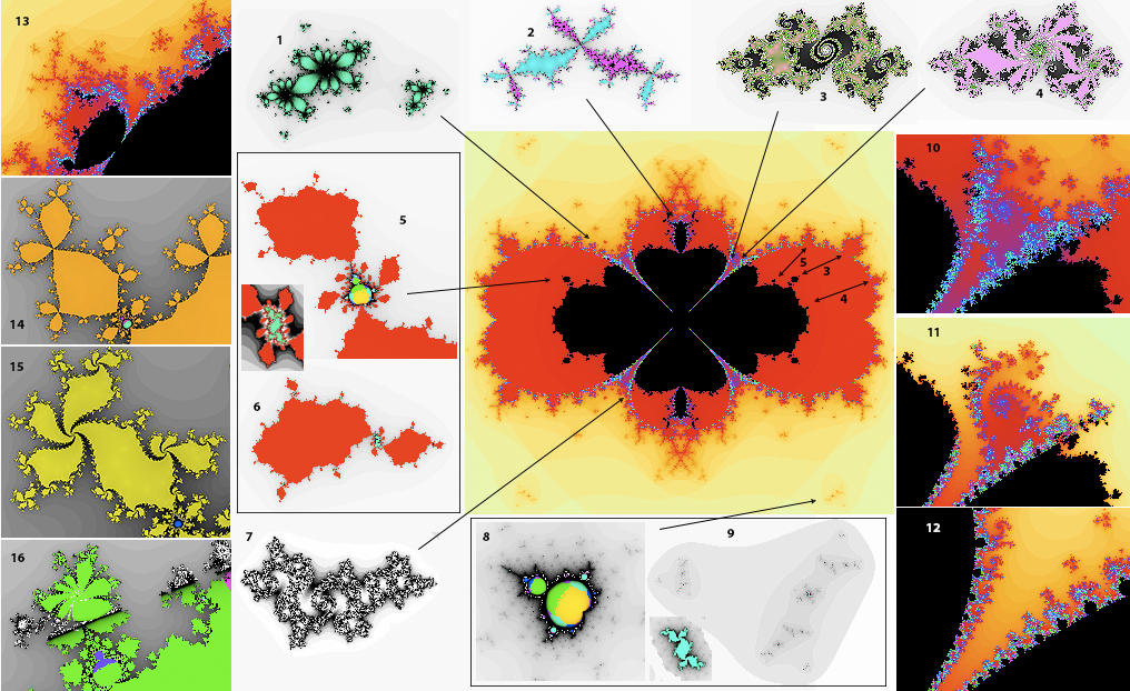
Fig 5: Dynamics of the function ![]()
Fig 5 (1-12) shows a variety of new
features which enter into the chaos with ![]() . The double parameter plane now has both black regions where
the Julia set is connected, orange regions where there is a fractal disconnect
in one of the factors and a light yellow exterior where both are disconnected.
Julia sets above illustrate (1) a single disconnection with the other factor of
period 9, (2) a connected set with two different periods, (3, 4) two sets in
the right hand cleft with rapidly changing dynamics between the two, (6) a
doubly connected Julia set of period 3 at a Mandelbrot satellite on the rocky
coastline of the black set and (7) a set on the edge of the lower cleft
dendritic on one factor and disconnected on the other.
. The double parameter plane now has both black regions where
the Julia set is connected, orange regions where there is a fractal disconnect
in one of the factors and a light yellow exterior where both are disconnected.
Julia sets above illustrate (1) a single disconnection with the other factor of
period 9, (2) a connected set with two different periods, (3, 4) two sets in
the right hand cleft with rapidly changing dynamics between the two, (6) a
doubly connected Julia set of period 3 at a Mandelbrot satellite on the rocky
coastline of the black set and (7) a set on the edge of the lower cleft
dendritic on one factor and disconnected on the other.
.
Julia journeys in an out of the Mariana trench.
Critical point co-Interference: Two major new features also arise.
The first is interference between the dynamics of the two critical points. In
each of the 'Mariana' trenches formed by the four deep cusps the higher and
higher periodicities of each are being perturbed by the other, fragmenting the
bulbs of each and leading to a newly chaotic dynamic, reminiscent of the
mode-locking perturbations that have thrown all the asteroids in any sort of
periodic relationship with the orbit of Jupiter into the other planets. In
(10-12) we can see blow-ups of the two separate parameter planes which not only
show chaos in superposition but each on its own is responding to the
perturbations of the other. This results in extremely small changes in the c values strongly altering the
relationship between the periodicities in the Julia sets.
Also the Mandelbrot satellites are no longer confined to dendrites but can also be connected through solid regions on the inner boundary where the bulbs are replaced by rocky coastline dark hearts, as on the dendrites of the quadratic case, except now attached to the main body via the cusps. (13-16) for k=0.2 show the erosion of higher period bulbs as k increases, with concretion of dendrites to periods 3, 4 and 8 due to a dominant periodicity on one critical point as for period 1 in (5,6).
![]() , each of which is shown in figs
4 and 5. The period 3 cubic double bulb and its satellites separate, with (a)
the left lobe in the movie becoming the dark hearts on the rocky inner
coastline of the distant critical point and (b) the right lobe becoming the
outer bulbs of the nearer critical point. The same picture applies to the cubic
satellites on the dendrites, the right set splitting to become (a) the dark
hearts on the smaller fractal rocks of the inner coastline defined by the
distant critical and (b) the dark heart islands of the nearer critical, with the
the left set splitting, with one set (a) descending to the adjacent rocky
coastline of the distant critical as the left lobe did, and the other (b)
continuing as outer bulb dendritic satellites. The dark hearts of each critical
point, being nuclei of attractive winding periodicities, are atomically robust
to interference from the other critical point and pass unaltered through such
changes, while their associated repelling dendrites become perturbed and undergo
bifurcation through an irrational flow to a base period Julia component. The
fractal rocks on the coastline associated with each dark heart thus originate
from the concretion of dendritic webs that have become frozen to the main body
attracting period of the other (adjacent) critical point.
, each of which is shown in figs
4 and 5. The period 3 cubic double bulb and its satellites separate, with (a)
the left lobe in the movie becoming the dark hearts on the rocky inner
coastline of the distant critical point and (b) the right lobe becoming the
outer bulbs of the nearer critical point. The same picture applies to the cubic
satellites on the dendrites, the right set splitting to become (a) the dark
hearts on the smaller fractal rocks of the inner coastline defined by the
distant critical and (b) the dark heart islands of the nearer critical, with the
the left set splitting, with one set (a) descending to the adjacent rocky
coastline of the distant critical as the left lobe did, and the other (b)
continuing as outer bulb dendritic satellites. The dark hearts of each critical
point, being nuclei of attractive winding periodicities, are atomically robust
to interference from the other critical point and pass unaltered through such
changes, while their associated repelling dendrites become perturbed and undergo
bifurcation through an irrational flow to a base period Julia component. The
fractal rocks on the coastline associated with each dark heart thus originate
from the concretion of dendritic webs that have become frozen to the main body
attracting period of the other (adjacent) critical point.
How the two halves of the period 3 bulb of z3+c separate into an outer bulb and a dark heart of z3-z+c,
with Julia journeys showing off mode 1's capacity to model periods, Cantor sets of escaping flows and irrational rotations.
The above movie shows how these phenomena arise as we move from f(z) =z3+c to f(z) =z3-z+c, each of which is shown in figs
4 and 5. The period 3 cubic double bulb and its satellites separate, with (a)
the left lobe in the movie becoming the dark hearts on the rocky inner
coastline of the distant critical point and (b) the right lobe becoming the
outer bulbs of the nearer critical point. The same picture applies to the cubic
satellites on the dendrites, the right set splitting to become (a) the dark
hearts on the smaller fractal rocks of the inner coastline defined by the
distant critical and (b) the dark heart islands of the nearer critical with the
the left set splitting with one set (a) descending to the adjacent rocky
coastline of the distant critical as the left lobe did, and the other (b)
continuing as outer bulb dendritic satellites. The dark hearts of each critical
point, being nuclei of attractive winding periodicities, are atomically robust
to interference from the other critical point and pass unaltered through such
changes, while their associated repelling dendrites become perturbed and undergo
bifurcation through an irrational flow to a base period Julia component. The
fractal rocks on the coastline associated with each dark heart thus originate
from the concretion of dendritic webs that have become frozen to the main body
attracting period of the other (adjacent) critical point.

Fig 5b: Per1(0),
Per2(0), Per3(0), colour coded by period, with five pre-periodic examples and
the Neut(λ) plane of Siegel discs, with example Julia sets. These can be accessed as special cases under rational in the help file.
Now let’s turn to the ‘slice’
method of investigating higher degree Julia sets favoured by classical
research. In figure 5b are shown slices of the 4D so-called cubic connectivity
locus which fix one critical point to periods 1, 2 and 3. These are highlighted
in mode 1 to emphasize their local conjugacy with the dynamics of the Julia
sets. We can easily confirm that the illustrated function
![]() has a
super-attracting fixed critical at 0, (derivative 0 with
period 1 hence Per1(0)), causing
has a
super-attracting fixed critical at 0, (derivative 0 with
period 1 hence Per1(0)), causing
![]() . Now let’s stipulate that
. Now let’s stipulate that
![]() , so that we have
, so that we have ![]() , giving
, giving ![]() . This has the parameter plane shown in fig 5b top right, with
dark hearts suspended in period 2 domains. The selected Julia sets
for several values of c show that
one critical point component of the dynamic is period 2 while the other can
take any configuration, from period 3 through Cantor dust to compound period 2
configurations. As shown lower left in fig 5b
we can do likewise for period 3 with
. This has the parameter plane shown in fig 5b top right, with
dark hearts suspended in period 2 domains. The selected Julia sets
for several values of c show that
one critical point component of the dynamic is period 2 while the other can
take any configuration, from period 3 through Cantor dust to compound period 2
configurations. As shown lower left in fig 5b
we can do likewise for period 3 with ![]() , resulting in the parametrization
, resulting in the parametrization
![]() , giving rise to a spectrum of locations. all of which have
one critical point inducing period 3 dynamics.
, giving rise to a spectrum of locations. all of which have
one critical point inducing period 3 dynamics.
![]() , with parametrization
, with parametrization ![]() . Complexity increases rapidly, so for
. Complexity increases rapidly, so for ![]() in PrePer(2,2)
in PrePer(2,2) ![]() giving rise to branch cuts and multiple parameter planes. These cases give rise to Julia sets with dendrites, tails and geometrical doublings.
giving rise to branch cuts and multiple parameter planes. These cases give rise to Julia sets with dendrites, tails and geometrical doublings.
Dark Heart also includes the period 4 case, ![]() which is right on the limits of computability, generating a 42 page formula in Mathematica after Matlab froze, which when computationally streamlined results in four multiply split parameter planes, generating a comprehensive collection of
period 4 coupled Julia sets. In fig 5c is shown the superimposed parameter
planes with selected Julia sets. The equations of the splits cannot be computed
as they are of degree greater than five.
which is right on the limits of computability, generating a 42 page formula in Mathematica after Matlab froze, which when computationally streamlined results in four multiply split parameter planes, generating a comprehensive collection of
period 4 coupled Julia sets. In fig 5c is shown the superimposed parameter
planes with selected Julia sets. The equations of the splits cannot be computed
as they are of degree greater than five.
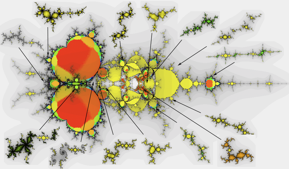
Fig 5c:
Four parameter planes of Per4(0)
superimposed, with a selection of Julia sets. This set can be exploredin rational 20 - see help file..
The last example
right in fig 5b examines the parameter plane Neut(λ) of
![]() , the golden mean value, which forces one critical point to give
rise to a neutral point rotation of a Siegel disc, while the other can vary at
will, as illustrated in the various Siegel discs both continuous and
discontinuous, one harbouring a complementary period 3 component. Rational
values can likewise be chosen for gamma resulting in parabolic examples. Again
this parameter plane has domains conjugate to Siegel discs. In the case gamma is a Cremer point, this
parameter plane is connected but not locally connected (Buff & Henricksen
2001), due to it being quasi-conformal with quadratic Julia sets of the form
, the golden mean value, which forces one critical point to give
rise to a neutral point rotation of a Siegel disc, while the other can vary at
will, as illustrated in the various Siegel discs both continuous and
discontinuous, one harbouring a complementary period 3 component. Rational
values can likewise be chosen for gamma resulting in parabolic examples. Again
this parameter plane has domains conjugate to Siegel discs. In the case gamma is a Cremer point, this
parameter plane is connected but not locally connected (Buff & Henricksen
2001), due to it being quasi-conformal with quadratic Julia sets of the form
![]() .
.

Fig 5d: The quasi-degenerate slice ![]() (Parameter file in quintics) has the
critical point at 0 mapped into the other at 2/3, resulting in a parameter
plane with bulbs having ‘quartic’ double cusps.
(Parameter file in quintics) has the
critical point at 0 mapped into the other at 2/3, resulting in a parameter
plane with bulbs having ‘quartic’ double cusps.
Higher Polynomials
Dark Heart extends the cubic
example to a series of higher degree functions, which can be modified in the
advanced settings to both change the degree and alter the separations between
critical points, leading to a huge diversity of examples. Application scripts
are also provided which can portray any polynomial up to degree 5 either in
terms of its coefficients, by solving for the critical points, or by setting the
positions of each of the four critical points and calculating the coefficients.
Several of the examples in advanced settings with symmetries can go to higher
degrees and also have negative powers, leading to infinite singularities.

Fig 6: Dynamics of higher degree polynomials
illustrating overlapping parameter planes, graded disconnections
and multiple Julia dynamical systems.
In fig 6 we examine
f(z) = z7 – 0.5z + c with a cascade of five dark hearts in successive rocky
coastlines, ending in a quadratic bulb, illustrating six stages in the fragmentation
of a degree seven Julia set, with the seventh stage being a completely disconnected Cantor
dust. On the right are blow-ups of
![]() showing multiple interference zones yielding Julia
sets below, each of which show the interaction of four dynamical systems. For
example, in the lower one, we have three periodic systems in green red and pink
and a Cantor dust disconnection of the multiple 'violins'.
showing multiple interference zones yielding Julia
sets below, each of which show the interaction of four dynamical systems. For
example, in the lower one, we have three periodic systems in green red and pink
and a Cantor dust disconnection of the multiple 'violins'.
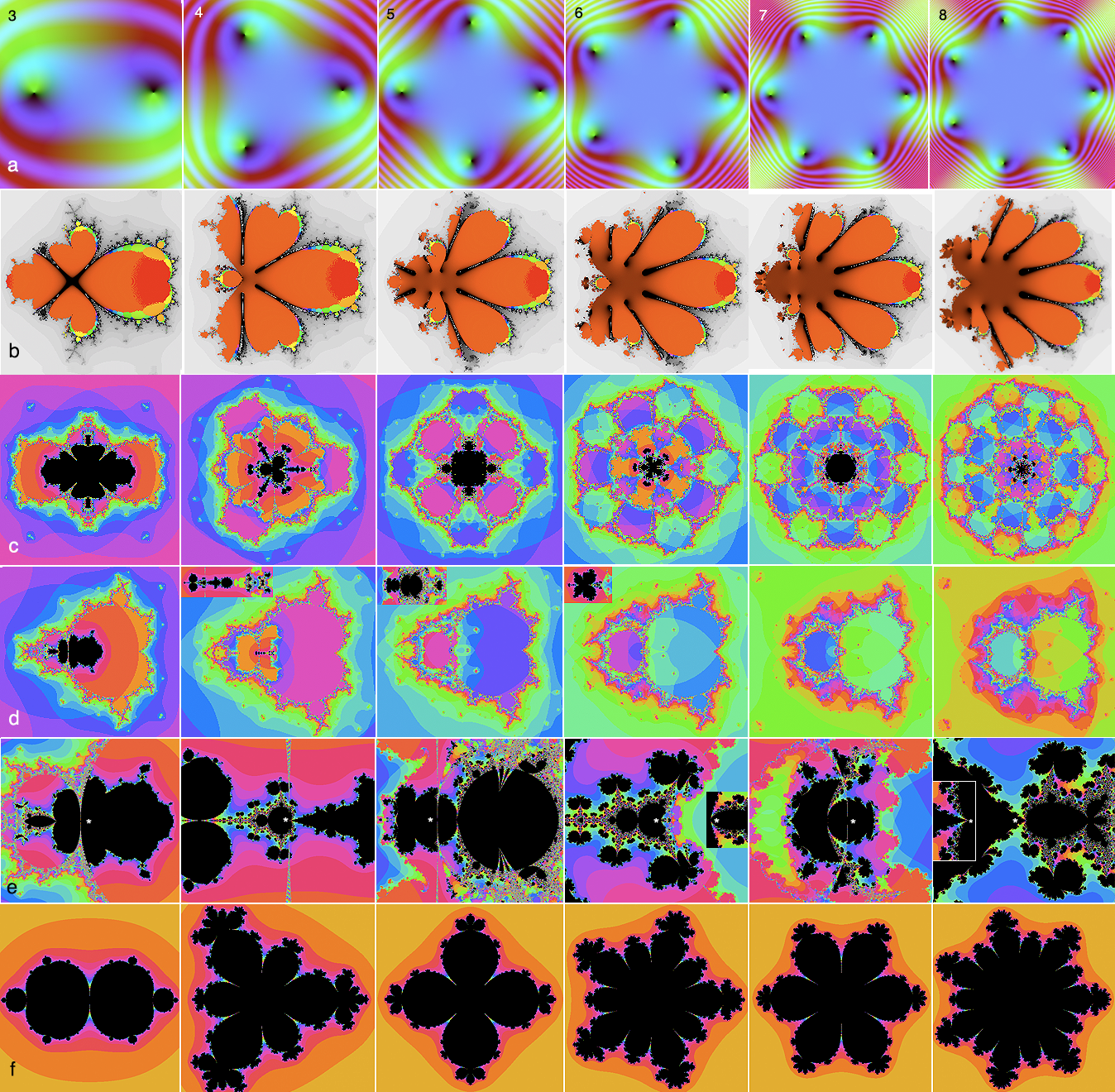
Fig 6b: Symmetries in polynomial dynamics of f(z) = zk - z + c for k = 3-8. One can use z^m-nz+c, and (z^m-n)(z+c) in modes 3, 6 or 7 with orbit trap selected to explore moduli spaces.
In fig 6b we explore the effects of symmetry, the use of
moduli spaces and the dynamics of odd and even powers. The polynomials f(z) = zk – nz are
unique in that they give rise to symmetric parameter planes. For n = 1, for every k the functions f(z) = zk - z + c have parabolic Julia sets at the origin, with
multiple cusps and petals, in bifurcation between periods 1 and 2. We can see
this because |f’(z)| = |kxk-1 - 1| =
1 for z = 0,
so 0 is on the boundary of the period 1 basin. In (a) the positions of the
critical points show that for even k,
the odd number of k-1 critical points
means that none are diametrically opposite one another, while in the odd case
the even k-1 criticals are opposite.
This leads to completely distinct Julia dynamics, in which for odd k we have k-1 petals, but for k even, we have 2(k-1), as illustrated
in (f). We can see why this is this in (b) when we examine the individual
parameter planes of each critical point for even k and find they have an intact period 2 basin opposite the main
period 1 basin, ecause there is no diametrially opposite critical point the the
rotational interference of the others tend to cancel, while the odd k have rocky coastlines there due to
interference from the antipodean critical, as we noted for k = 3 in fig 5. In the even case, this causes the central (black)
region where the Julia sets are fully connected (c) to be ‘stellated’ and split
by multiple cusps from the adjacent period 2 basin. In the odd case we have a
central region punctuated only by the global cusps of the remote period 1
basin, which we can see intersecting for k = 3, but gradually become invisible for higher powers.
We can explore this further, by explitiong the symmetry of
the functions by a rotation by 1/(k-1)
of a revolution when the overlapping parameter planes are combined, as shown in
(c). We can thus introduce a mapping to another C-plane, where C = c1/(k-1) , to form the moduli space of
equaivalence classes of c under the
rotational symmetry, as illustrated in (d). In particular, this transformation
is a Mobius transformation ![]() which conjugates with the polynomial function, so we can
generate its own parameter plane which in each case now looks like a set of overlapping dark hearts. This
perfectly represents all the possible Julia sets up to rotation by 1/(k-1) of a revolution, but it also
involves geometrical scaling so that for higher values of k the black region (inset for k = 4-6) becomes shrunken and
distorted about the origin, while preserving the fractal sturctures and topological
dynamics completely.
which conjugates with the polynomial function, so we can
generate its own parameter plane which in each case now looks like a set of overlapping dark hearts. This
perfectly represents all the possible Julia sets up to rotation by 1/(k-1) of a revolution, but it also
involves geometrical scaling so that for higher values of k the black region (inset for k = 4-6) becomes shrunken and
distorted about the origin, while preserving the fractal sturctures and topological
dynamics completely.
When we examine the cases in (d), we see that for even k, the origin is always at a cusp in a
dark heart region penetrated by a complementary region, while in the odd case
we find a central region penetrated only by the universal vertical cusps of the
remote period 1 basin.
Separations of the above degree 3 to 5 polynomials from their atoms
Rational Functions and Infinities
There are also an intriguing
array of rational functions which have infinite singularities as well as
critical points which disturb the dynamics in sometimes un predictable ways and
which provide new interesting dynamical examples.
A famous one is Newton's method
in which we find the zeros of a function by iterating from a start point x , going up to f(x) and then down the
slope f'(x) to the point ![]() . Virtually always this closes in on the zero but not every time. There is a chaotic set of points that can't decide what to do and we can explore it for the complex cube roots of unity. It turns out that we can describe any cubic in the form
. Virtually always this closes in on the zero but not every time. There is a chaotic set of points that can't decide what to do and we can explore it for the complex cube roots of unity. It turns out that we can describe any cubic in the form ![]() . Dark Heart applies this generalized to
. Dark Heart applies this generalized to ![]() to get Newton's method for the
complex k-th roots of unity. In fig 7
the parameter plane of Newton on the fifth roots of unity is shown (1),
iterated from the repelling critical point at 0. This puts the origin on the
chaotic Julia set, but other c values
not on the Julia set mostly iterate into one of the five attracting roots. (2)
shows a parameter plane blow up with a degree-4 Mandelbrot kernel, and (3) the
Julia set of the iteration for c = 1,
to the fifth roots one in each of the large colour-coded regions with fractal replicates eventually mapping onto these. This provides a unique fractal 5-colour mapping problem in
which every point on the boundary of each region is simultaneously touching all
of the other four regions because every boundary point is a fractal boundary
intersection point of all regions.
to get Newton's method for the
complex k-th roots of unity. In fig 7
the parameter plane of Newton on the fifth roots of unity is shown (1),
iterated from the repelling critical point at 0. This puts the origin on the
chaotic Julia set, but other c values
not on the Julia set mostly iterate into one of the five attracting roots. (2)
shows a parameter plane blow up with a degree-4 Mandelbrot kernel, and (3) the
Julia set of the iteration for c = 1,
to the fifth roots one in each of the large colour-coded regions with fractal replicates eventually mapping onto these. This provides a unique fractal 5-colour mapping problem in
which every point on the boundary of each region is simultaneously touching all
of the other four regions because every boundary point is a fractal boundary
intersection point of all regions.
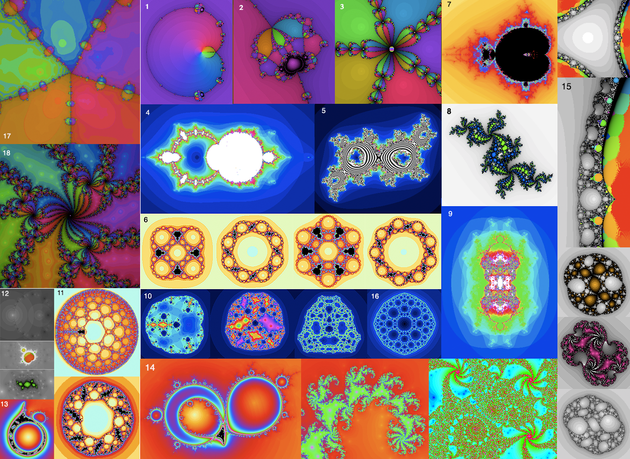
Fig 7: Varieties of rational function dynamics
In (4) is the parameter plane of![]() , which for golden mean rotations in the left sector,
provides the Herman ring - a unique example of an annular irrational flow in
the Julia set (5). Notice also
that the left hand portion of the parameter plane surrounding the singularity
has both inward and outward pointing bulbs, leading to inversions of the Julia
set dynamics.
, which for golden mean rotations in the left sector,
provides the Herman ring - a unique example of an annular irrational flow in
the Julia set (5). Notice also
that the left hand portion of the parameter plane surrounding the singularity
has both inward and outward pointing bulbs, leading to inversions of the Julia
set dynamics.
In (6) parameter planes and
Julia sets for ![]() provide an example of symmetries generated by each of the two
powers. In the (5,3) case there are 5-1=4 baby dark hearts.
Each of the intervening 4 concentric domains has 5+1 outer sub-domains and
3-1=2 inner sub-domains adding to the 5+3=8 fold rotational symmetry of the
Julia sets with 5 outer and three inner sub-domains.
provide an example of symmetries generated by each of the two
powers. In the (5,3) case there are 5-1=4 baby dark hearts.
Each of the intervening 4 concentric domains has 5+1 outer sub-domains and
3-1=2 inner sub-domains adding to the 5+3=8 fold rotational symmetry of the
Julia sets with 5 outer and three inner sub-domains.
Filigree journeys around z3+n/z for small n.
Another intriguing phenomenon is the way a
singularity can introduce fractal perforations in an existing iteration. In (7)
the parameter plane of
![]() shows the dark heart perforated in the centre by the effect
of the singularity, which has also fragmented the critical points into a
closely spaced set of 3, generating overlapping parameter planes. A Julia set
from the period 3 bulb (8) shows internal perforation by a latticework of
'holes' with multiple dynamical systems in the interior due to the multiple
critical points. In (9) the iteration
shows the dark heart perforated in the centre by the effect
of the singularity, which has also fragmented the critical points into a
closely spaced set of 3, generating overlapping parameter planes. A Julia set
from the period 3 bulb (8) shows internal perforation by a latticework of
'holes' with multiple dynamical systems in the interior due to the multiple
critical points. In (9) the iteration
![]() shows almost
completely scrambled parameter planes generating the diverse Julia sets shown
in (10).
shows almost
completely scrambled parameter planes generating the diverse Julia sets shown
in (10).
(11) Shows
![]() and a Julia set
of period 3, with similar power-based symmetries to (6). You can also see here the corresponding Mandelbrot and Julia sets for cz2(1-z)n n=5,7 displaying even closer affinity with hyperbolic space due to the fractional rotation of the second factor. Notice the patterns in the bottom left Mandelbrot set whose dark hearts are so relatively tiny(the actual set is 80000 across) that you can see them only in the inset centre. Notice that while the lower right Julia figure has islands growing by 3*2n ... 3, 6,12 etc. the Mandelbrot figure lower left grows by 2+1+2+4+8 ... or 2n+1 ... giving 3, 5, 9, 17 etc.
and a Julia set
of period 3, with similar power-based symmetries to (6). You can also see here the corresponding Mandelbrot and Julia sets for cz2(1-z)n n=5,7 displaying even closer affinity with hyperbolic space due to the fractional rotation of the second factor. Notice the patterns in the bottom left Mandelbrot set whose dark hearts are so relatively tiny(the actual set is 80000 across) that you can see them only in the inset centre. Notice that while the lower right Julia figure has islands growing by 3*2n ... 3, 6,12 etc. the Mandelbrot figure lower left grows by 2+1+2+4+8 ... or 2n+1 ... giving 3, 5, 9, 17 etc.
(12) shows the ghostly outlines of the repelling version of
Newton’s method
![]() , dominated by escaping points, leaving only isolated regions
of connectivity, with a Mandelbrot island of base period 2 and a period 6 Julia
set.
, dominated by escaping points, leaving only isolated regions
of connectivity, with a Mandelbrot island of base period 2 and a period 6 Julia
set.
![]() using the Milnor
C-script and function. (15) Shows the parameter plane and Julia sets of
using the Milnor
C-script and function. (15) Shows the parameter plane and Julia sets of ![]() . Several of the functions in advanced settings
admit singularities from negative powers of z so there is a good library of varied rational functions. (16) Shows the Julia set of f(z) = z2 + (1/16) z-2 is a Sierpinski carpet. (17,18) Julia sets of c(z+1/z+2)+1 (Mandel1.txt in milnor) and c(z+0.5/z2) (Rational 23) showing internal dynamics and fractal tilings of the complex plane in mode 3 showing how the attractors separate the plane into fractal tilings (Parameter files in rational fig7-17, 18).
. Several of the functions in advanced settings
admit singularities from negative powers of z so there is a good library of varied rational functions. (16) Shows the Julia set of f(z) = z2 + (1/16) z-2 is a Sierpinski carpet. (17,18) Julia sets of c(z+1/z+2)+1 (Mandel1.txt in milnor) and c(z+0.5/z2) (Rational 23) showing internal dynamics and fractal tilings of the complex plane in mode 3 showing how the attractors separate the plane into fractal tilings (Parameter files in rational fig7-17, 18).


Light at the end of the tunnel – three 1255 x 677 images of Julia sets of c(z+0.5/z2)
Both cubic polynomials and quadratic rational
functions have two critical points, where the derivative is zero or infinite,
leading to a 4D moduli space (2 complex parameters), under equivalence by
Mobius transformations, to completely describe the Julia sets of every
function. However, as we have seen with cubics, it is possible to form a slice consisting of functions fixing the behavior of one critical point, to form a 2D
parameter plane constituting a section through the higher dimensional space, in
which the remaining critical point is set free and we can study the dynamics of
the Julia sets. The critical points can have one of four behaviors adjacent if they both fall into the same
attracting set, bitransitive if each falls into the others basin, capture if one falls into the
periodicity of the other and disjoint if they have entirely separate basins of attraction. The k periodic regions of the infinite component differ in their
behaviours. For example the main light-coloured bulb in Per2(0) in fig 7b has adjacent behaviour. Each successive
period 2 generation daughter reverses between this and bitransitive.
We thus fix the period of one critical and find a parametric class of functions all of which preserve the periodicity. In fig 7b are shown representative parameter planes Perk(0) k=1-4 for the sections fixing the periodicity of the critical point z = 0, corresponding to the following four parametrizations:
![]()
The first is chosen to be the quadratic Mandelbrot set because it has fixed critical point zero and a super-attractor at infinity (the north pole of the Riemann sphere), leading to an infinite period one basin (enclosing the northern hemisphere) surrounding the Julia set.
In the period two case,
![]() . In period 3,
. In period 3,
![]() using
using ![]() , giving the above equation, with critical points at 0 and
infinity. This provides symmetric Julia sets rather than the asymmetric
model based on
, giving the above equation, with critical points at 0 and
infinity. This provides symmetric Julia sets rather than the asymmetric
model based on
![]() .
.
The symmetrical period 4 case is special because
it has a square root in the c parameter defining f, which
leads to a double split parameter plane, generating the two parameter planes shown
in the third row of fig 7b forming a “fermionic” loop where one cycle through
the elliptical cut in the centre of the each plane takes you to the
complementary plane. Together these planes cover all the period 4 locations on
the classical Mandelbrot set, as shown on the left. There is also a topological
homology between the Julia sets generated by Medusa and those generated by the
fermionic plane, as shown in the second and fourth rows of fig 7b.
The period 4 case is special because it has a
square root in the c parameter defining f, which
leads to a double-split parameter plane, generating two parameter planes shown
in the third row of fig 7b forming a “fermionic” loop
where one cycle through the elliptical cut in the centre of the plane on the right in fig 7b takes you to the complementary plane.
Together these planes cover all the period 4 locations on the classical
Mandelbrot set, as shown on the left. There is also a topological homology
between the Julia sets generated by Medusa and those generated by the fermionic plane, as shown in the second and
fourth rows of fig 7b.
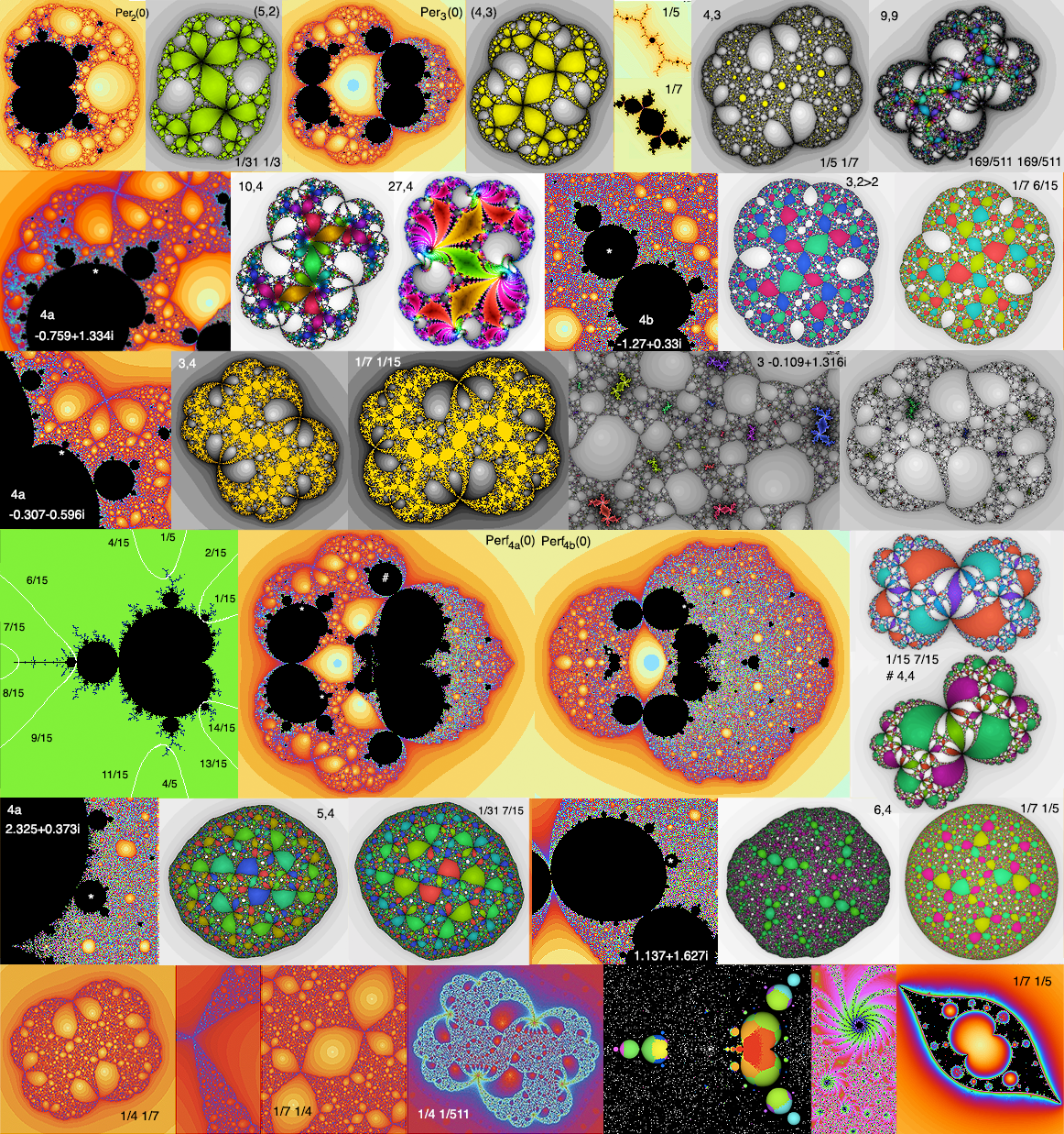
Fig 7b: Top row: Periodic 2 and 3
slices and Julia set matings. Right: Two Medusa matings. The lower three rows show the split parameter plane Perf4(0),
with Julia sets at the starred locations, showing topological homology with corresponding Medusa matings (3,2>2 <-> 1/7 6/15, 5,4 <-> 1/31 7/15, 3,4 <-> 1/7 1/15 and 4,4 1/15 7/15) confirming the
techniques can generate conjugate dynamical systems of shared matings although the parameter lanes are generated in completely different ways.
Each parameter plane gives rise to
Julia sets, in which a new phenomenon, called mating appears. You can think of a quadratic rational function as
the quotient of two quadratics, one of which has dynamics
which is dominant near zero with the other dominant near infinity. Because
the complement of a connected quadratic Julia set is a topological disc, two connected
Julia sets can be entwined together on opposite hemispheres of the Riemann
sphere. Consequently they can form complementary Julia sets “mated” together. Almost
any pair of connected Julia sets can be so mated except for those in conjugate
limbs of the Mandelbrot set. Thus we can see that the boundary of a mated Julia
set is penetrated by periodic basins, as well as having periodicities of its
own, just like the period 2, 3 and 9 basins in the top row with inner Julia components of period 5, 4, 4 and 9 respectively.
Mating is an extension of the picture we saw with cubic polynomials where the Julia sets had two fractal components, one corresponding to each critical point. A mating simply moves the two critical points around to be at or close to 0 and ∞.

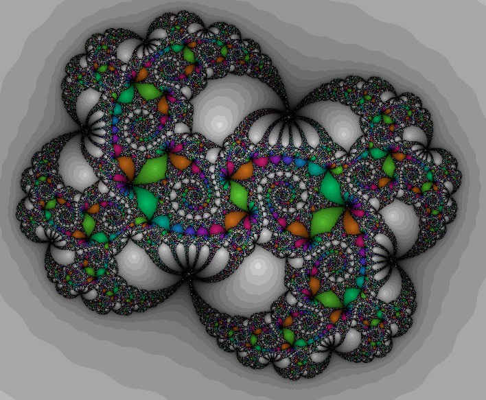

Fig 7b2: Medusa matings for 1/255 63/255, 1/255 1/255 and 1/255 3/7.
The
Medusa algorithm to find a rational function, which mates two rational Julia
sets of any pair of external angles p/q and r/s, (Boyd & Henriksen 2012) uses the combinatorics of a spider consisting of a set of periodic
points and external angle rays in the orbit of the critical point c. A medusa consists of two spiders
forming northern and southern hemispheres of the Riemann sphere sewn together
along the equator.
![]() mating the
Julia sets defined by the two external angles. Note that if the coefficients give an infinite Julia set (initally black but with escape only off it becomes visible and unbounded), one can use (1-b, 1-a) in the place of (a, b) to get a finite Julia set, as 1/f1-b,1-a(1/z) = fa,b(z). You can use the Wolf Jung's Mandel app included with the package to find where the external rays meet the Mandelbrot set geometrically to decide the Medusa fractions to explore. Period k bulbs and Mandelbrot satellites have rays with fractions n / (2k-1). The Medusa iteration may diverge or remain unstable for some fractional angles, including some with even denominators. As shown in fig 7b many Medusa matings are visually and topologically identical to those of slices, but some are subtly different because Medusa throws up an equivalent or shared mating, such as the period 4 Julia denoted with a # in fig 7b.
mating the
Julia sets defined by the two external angles. Note that if the coefficients give an infinite Julia set (initally black but with escape only off it becomes visible and unbounded), one can use (1-b, 1-a) in the place of (a, b) to get a finite Julia set, as 1/f1-b,1-a(1/z) = fa,b(z). You can use the Wolf Jung's Mandel app included with the package to find where the external rays meet the Mandelbrot set geometrically to decide the Medusa fractions to explore. Period k bulbs and Mandelbrot satellites have rays with fractions n / (2k-1). The Medusa iteration may diverge or remain unstable for some fractional angles, including some with even denominators. As shown in fig 7b many Medusa matings are visually and topologically identical to those of slices, but some are subtly different because Medusa throws up an equivalent or shared mating, such as the period 4 Julia denoted with a # in fig 7b.
Medusa can also generate matings involving dendritic Julia sets by using external rays with even fractions, landing on the intersection points of repelling dendrites, as shown in the bottom row of fig 7b. Notice that 1/7 1/4 has an unbounded Julia set because the point at infinity is on a dendrite. One can also generate sets like 1/4 1/7 by selecting an appropriate c value in Per3(0). To generate sets like 1/7 1/4, we need to construct a pre-periodic parameter plane. In
fig 7b is shown the pre-periodic slice PrePer(2,1)
![]() ,
,


Fig 7b3 Click each image to see video: Three movies generated by Claude's algorithm show: (a) Basilica (-1,0) with Rabbit (-0.122 0.75), (b) Pd 3 satellite (-1.75,0) with Pd 3 dendrite (-0.101096,0.95629) (c) Pd 5 dendrite (-0.6702, 0.45806) with Pd 3 dendrite (-0.101096,0.95629), portrayed on a cylindrical presentation of the Riemann sphere, to show their interaction symmetrically, rather than the planar presentations used above.
The Slow Mating algorithm. There is a second method of deriving matings called "slow mating", in which we start with two locally-connected Julia sets, each having a complementary disc in the Riemann sphere. Since all their external potential function level sets are Jordan curves (topological circles) we can glue a level set of one to a corresponding level set of the other along their boundaries. By moving the gluing to successively closer potential levels, the Julia sets approach one another more and more intimately, until a mating ensues, when we reach their conjoined boundaries. This method requires mapping the fractal Jordan curve of each and pulling one back to the complementary disc of the other. so it is computationally subtle. It also gives very good movie images when we are trying to observe matings between two dentriditc Julia sets, where the mated condition is densely interconnected. Arnaud Cheritat has some good videos of this method, but lacks the supporting code, leading to Claude Heiland-Allen's code being generated to nicely fill the gap in cylndrical rather then spherical presentation.
The status of Julia set mating for higher powers than quadratic is a more complex question. However there is one form of degree four situation called "anti-mating". Here tthe both composites of 2 quadratic functions P(z) = z2+p and Q(z)= z2+q are taken to make two related Julia sets. It then proves straightforward to perform a slow mating of the two composites P(Q(z)) and Q(P(z) in the same way as above.
Finally it is possible to have equivalent matings of Julia sets generated from different periodic regions in the quadratic paramter plane with differing external angles, such as 3/15 3/7 between satellite Mandelbrots has Julia sets which are simply rotated versions of those of
1/7 6/15 arising from period 3 and 6 bulbs. Other Julia sets which may appear to have a distinct fractal geometry may also be topologically equivalent and hence shared matings.
A more detailed comparison of the actual matings (pdf).

Fig 7c: Dynamics of the function ![]() with both finite and
infinite critical points.
Parameter files for (7) and (9) are included which can also be used to fully explore the example.
with both finite and
infinite critical points.
Parameter files for (7) and (9) are included which can also be used to fully explore the example.
The slice
function
![]() in fig 7c
demonstrates the dynamics when we have to take account of both the critical points
with zero derivative and those with an infinite derivative. Here we have
in fig 7c
demonstrates the dynamics when we have to take account of both the critical points
with zero derivative and those with an infinite derivative. Here we have
![]() and since
and since
![]() , we can effectively use 0 and 1 as the critical points. Moreover,
we can see by swapping 0 and ∞ by
, we can effectively use 0 and 1 as the critical points. Moreover,
we can see by swapping 0 and ∞ by
![]() in both the
domain and range that
in both the
domain and range that ![]() , so the parameter plane of ∞ is simply the parameter plane
of 0 flipped in the c direction. This results in the
combined plane shown in (1), with the two individual planes in (3,4). The
combined plane forms a symmetrical figure 8 with pairs of bulbs running in two
series (2) in the interior of the black chaotic region, which consists of
points which fail to head to any attractor from either critical point.
, so the parameter plane of ∞ is simply the parameter plane
of 0 flipped in the c direction. This results in the
combined plane shown in (1), with the two individual planes in (3,4). The
combined plane forms a symmetrical figure 8 with pairs of bulbs running in two
series (2) in the interior of the black chaotic region, which consists of
points which fail to head to any attractor from either critical point.
Close
inspection however reveals that, the two, apparently symmetrical, sides differ. Superimposing the left and right for the
period-16 bulb (2i) shows that, although these overlap, there are key
differences. The expanded
superimposed period 13 and 16 bulbs (5,6) have clear patterns indicating
critical point interference. Intriguingly for the period 13 and 16 cases, the
bulb of 0 intersects both with regions of identical asymptotic period (13 or 16) in the bulb of
∞, and with c values where ∞ is pre-periodic, or chaotic and hence in the Julia set.
Note the two critical points differ fundamentally in their behavior, because one is a zero of the derivative which is not a solution of the numerator and the other is simply a solution of the denominator. This means that the Julia sets on either side have distinct dynamics.
As rational functions with a critical point at 0 and ∞, the Julia sets manifest as matings. (15,16) for example show complementary matings between a jagged period 3 Julia and a rounded period 2 Julia. In 15 on the left the exterior is partof the rounded Julia but the complementary Julia 16 on the right has a gagged exterior and rounded motifs internally. Similarly (17,18) display a 1,3 mating inverting to a 3,1 rabbit in the complementary set.
In
the above cases, when a c value is chosen, where both criticals have the same asymptotic period, as in (7,8 c = ±0.995627+1.937037i) and (9,10 c = ±0.731013+2.280174i), (Rational fn 24 - 3.1, parameter files in rational fig7c7, 9) the Julia sets on both sides,
although geometrically distinct, appear to be homeomorphic to one another and each is hence automorphic to itself,
by an inversion exchanging 0 and ∞, as indicated by a blow-up of the central
regions of (9,10) in (9b,10b). These thus appear to be automprphic matings.
However, if a pre-periodic point is picked in a bulb on either side (if c is picked on the left -c will have precisely the same effect and equivalent location on the right), the right-hand Julia sets will be fractal to 0 as in (11) and the left-hand Julia sets will become unbounded (fractal to ∞, as in (12). (13) & (14) show a value very close to the intersection of the Julia arcs lower-right in (5), giving a right-hand Julia with a double intersection very close to 0 and a left-hand Julia expanding toward infinity with a double 13 period array, confirming the general picture.

A single Mandelbrot bulb portal in the function![]() generates an infinite variety of Julia sets.
generates an infinite variety of Julia sets.
Portals frequently occur when the two parameter planes have coinciding internal bulbs, one of which has interference from the other critical point.
The function ![]() can be generalized to the functions
can be generalized to the functions ![]() and
and ![]() .
.
These can still be solved in the same way viz: ![]() , giving symmetric polygonal Julia sets and
, giving symmetric polygonal Julia sets and![]() where
where ![]() , which give rise to polygonal Julia sets with symmetry broken by the –z term. Hence we can still use 0 and 1 as the two critical points. Furthermore the parameter planes for varying powers of c give completely different Julia sets because the c exponents in the numerator and denominator of the function have differing powers and hence differing values for a given fixed c.
, which give rise to polygonal Julia sets with symmetry broken by the –z term. Hence we can still use 0 and 1 as the two critical points. Furthermore the parameter planes for varying powers of c give completely different Julia sets because the c exponents in the numerator and denominator of the function have differing powers and hence differing values for a given fixed c.
However the original case ![]() is the only case where the parameter plane has the semi-reflection property.
is the only case where the parameter plane has the semi-reflection property.
![]() because the only solutions of this equation, which reduces to the solutions of
because the only solutions of this equation, which reduces to the solutions of ![]() for integer powers m and n . These are (3,2), as above and (2,3), but the power of c also has to be odd so the signs of both c powers in the numerator and denominator flip, eliminating this last case.
for integer powers m and n . These are (3,2), as above and (2,3), but the power of c also has to be odd so the signs of both c powers in the numerator and denominator flip, eliminating this last case.
Figure 7d shows a variety of the parameter planes and Julia sets. These show the unique capacity to generate symmetry-broken higher-degree rational functions with perfect Mandelbrot and Julia sets.

Fig 7d: Varieties of Mandelbrot and Julia set of ![]() and
and ![]() High res image of x 100.
High res image of x 100.

Fig 7e: Examples with negative powers of z. In the latter three, effective degree 1 symmetry-breaking occurs
due to negative powers of z in the first term being dominated by the linear second term.
Functional Transcendence
Transcendental functions exp,
cos and sin expand the repertoire to include a variety of new phenomena. In fig
8 top row are (A) the escaping fronds of f(z) = ez + c with increasing periods colour
coded (B). The Mandelbrot set here is black. In (C) is the Julia set of ez/e. The
Fatou set here is in black. The Julia set, in colour, consists of an
uncountable infinity of closely packed disjoint curves of fractal dimension 2, forming
a Cantor bouquet. When the main basin has a higher period, the bouquet can
become pinched causing the curves to intersect, as in the period 3 example (D).
The exponential function, shown to have a plateau in fig 4 can be perturbed to
include polynomial critical points. In (1) is shown the parameter plane of
the critical point z = -1 of the
function
![]() , which has small clearly defined period 3 bulbs giving rise
to period 3 Julia sets (2). These also have green period 6 exponential bays resulting from the plateau critical at negative x, as indicated by the green fronds in the period 3 bulb (inset centre). When we change to the multiplicative version
, which has small clearly defined period 3 bulbs giving rise
to period 3 Julia sets (2). These also have green period 6 exponential bays resulting from the plateau critical at negative x, as indicated by the green fronds in the period 3 bulb (inset centre). When we change to the multiplicative version
![]() in (3) we find we have a local parameter plane very similar
to that of the polynomial cz(1-z)
illustrating the difference between additive parameter planes and
multiplicative ones, which operate more simply by scaling rather than
translation. A period 3 Julia set is shown in (4).
in (3) we find we have a local parameter plane very similar
to that of the polynomial cz(1-z)
illustrating the difference between additive parameter planes and
multiplicative ones, which operate more simply by scaling rather than
translation. A period 3 Julia set is shown in (4).
![]()
Fig 8: Transcendental parameter planes and Julia sets.
The trigonometric functions sin
and cos are combinations of rotated complex exponentials, which are themselves
periodic in the imaginary direction e.g.
![]() . By superimposing a positive and negative exponential we arrive
at a transcendental function with a chain of quadratic maxima and minima along
the x-axis and consequently the
parameter plane of
. By superimposing a positive and negative exponential we arrive
at a transcendental function with a chain of quadratic maxima and minima along
the x-axis and consequently the
parameter plane of
![]() (5) looks almost exactly like a chain of copies of the cubic
function in fig 5 with corresponding two factor Julia set kernels as shown in
(6). Rather than isolated Julia sets as we see in polynomials we now have
networks of kernels connected by dendrites, or in a Cantor set arrangement. In
(7) we see the multiplicative Mandelbrot set and a Julia set of
(5) looks almost exactly like a chain of copies of the cubic
function in fig 5 with corresponding two factor Julia set kernels as shown in
(6). Rather than isolated Julia sets as we see in polynomials we now have
networks of kernels connected by dendrites, or in a Cantor set arrangement. In
(7) we see the multiplicative Mandelbrot set and a Julia set of
![]() , which displays combined quadratic and quartic dynamics and
in (8) Superimposed Mandelbrot and a
, which displays combined quadratic and quartic dynamics and
in (8) Superimposed Mandelbrot and a
![]() , at c = 1.5
+ 0.15i, which shows three different
kernel types in a chain.
, at c = 1.5
+ 0.15i, which shows three different
kernel types in a chain.
.
Descending through the upper period 4 bulb of c(z-tan(z)).
To explore transcendentals with
both zeros and infinities, we now look for tractable functions involving the
tangent. The final example in (9) is the function ![]() , which has derivative
, which has derivative ![]() and thus has
alternating zeros and infinities of the derivative. Applying the zero
criticals, we arrive at (9) which like the Herman ring example of fig 7, has
inward and outward pointing bulbs due to the singularities. Examples of Julia
sets (a-c) show the dynamics. Note that the actual periodicities of the bulbs
to the left and right differ although the parameter plane is symmetric because
the winding involves realising inversions in one half but not the other,
resulting in different 'spirograph' periodicities in the ascending periods.
and thus has
alternating zeros and infinities of the derivative. Applying the zero
criticals, we arrive at (9) which like the Herman ring example of fig 7, has
inward and outward pointing bulbs due to the singularities. Examples of Julia
sets (a-c) show the dynamics. Note that the actual periodicities of the bulbs
to the left and right differ although the parameter plane is symmetric because
the winding involves realising inversions in one half but not the other,
resulting in different 'spirograph' periodicities in the ascending periods.![]() , showing rational
transcendental functions. (13) shows the parameter plane and Julia sets of f(z)=ccos(z1/2). Half-integer powers work seamlessly for the cosine
function because it has only even powers of z. The parameter plane and Julia sets of
, showing rational
transcendental functions. (13) shows the parameter plane and Julia sets of f(z)=ccos(z1/2). Half-integer powers work seamlessly for the cosine
function because it has only even powers of z. The parameter plane and Julia sets of
![]() are also shown in fig 10. (14) shows the logarithm f(z)=clog(z) which fractally splits the
complex plane, as do non-integer powers of z.
are also shown in fig 10. (14) shows the logarithm f(z)=clog(z) which fractally splits the
complex plane, as do non-integer powers of z.
Dark Heart contains a series of
further examples to explore various issues with transcendental functions. For
example attempts to produce other kinds of critical points than those of fig 4
appear to fail because Fourier transforms, such as those producing square or
triangular waves in the limit converge to a real function on the x-axis. Also included are log function
examples, which are not defined on the complex plane, but on a Riemann surface,
requiring the plane to be cut in a way which results in fractal spits in the
Mandelbrot and Julia sets. A complex function implementation of the Collatz 3n+1 problem is included.
The Ultimate Challenge: Zeta and L-functions
We now turn to the most challenging functions of all, those defined by Dirichlet series, requiring analytic continuation using gamma functions and Mellin integral transforms to put together a complete picture. I have designed Riemann Zeta viewer to specialize in these functions, including Riemann zeta, and the related eta, xi and Dirichlet and other L-functions, running right to the limits of current analytical number theoury research. This runs in the same way as Dark Heart but with some additionally focused controls.
The archetypal and most famous
example is the Riemann zeta function shown in fig 9 - 1(a). This has a single
infinity at x = 1 due to the harmonic series![]() , multiple (trivial) zeros along the negative x-axis due to the analytic continuation,
and a string of irregularly placed (non-trivial) zeros forming a kind of
Fourier transform of the primes along the critical line x=1/2.
, multiple (trivial) zeros along the negative x-axis due to the analytic continuation,
and a string of irregularly placed (non-trivial) zeros forming a kind of
Fourier transform of the primes along the critical line x=1/2.
The Riemann zeta function is
formally defined as either a sum over negative powers of the integers or an Euler product over the primes![]() . But neither definition is convergent to the left of 1, but can be analytically continued to the entire complex plane, using the gamma function
. But neither definition is convergent to the left of 1, but can be analytically continued to the entire complex plane, using the gamma function![]() - a generalization of n!
=n(n-1)…3.2.1 - to derive the functional equation
- a generalization of n!
=n(n-1)…3.2.1 - to derive the functional equation![]() expressing
values for z < 0 in terms of those
for z > 1. This would enable us to
produce a portrait were it not for the fact that in the critical strip 0 < z < 1 the function is still
divergent, so we have to resort to a trick, which is to use the fact that the
Euler eta function converges for z > 0 because it is an alternating series
expressing
values for z < 0 in terms of those
for z > 1. This would enable us to
produce a portrait were it not for the fact that in the critical strip 0 < z < 1 the function is still
divergent, so we have to resort to a trick, which is to use the fact that the
Euler eta function converges for z > 0 because it is an alternating series![]() and can be used
to represent zeta. So for zeta, we use eta to get zeta for z > 1/2 and use the functional equation to get 1 – z . i.e. z < 1/2.
and can be used
to represent zeta. So for zeta, we use eta to get zeta for z > 1/2 and use the functional equation to get 1 – z . i.e. z < 1/2.

Fig 9: Sample illustrations of parameter planes and Julia
sets of the Riemann zeta function.
In fig 9 1(a) is the zeta function showing
trivial x-axis zeros, non-trivial
on x = 1/2 zeros and the red infinity at z = 1. In (b) is the derivative of zeta showing the critical points. (c) shows the additive parameter plane![]() for the critical plateau z ~ 1000 showing sample Julia sets with the periods illustrated filling the right
half plane. In (d) is the multiplicative parameter plane is portrayed.
for the critical plateau z ~ 1000 showing sample Julia sets with the periods illustrated filling the right
half plane. In (d) is the multiplicative parameter plane is portrayed.
The four illustrations in (2) show the dark heart
at the end of the central valley for the critical point z = -17.3 along with a
sample period 3 Julia set, (3) the central basin with quadratic bulbs of
critical z = -15.33 and obvious cubic
interference similar to fig 5. (4) Details of the basin of the non-trivial
critical point around z = 1/2 + 95i exploring a satellite dark heart and
an associated period 3 Julia set, and (5) a dark heart in the singularity
island for the critical point z =
-13.29.
.
Explosions of the Riemann zeta Julia sets as c moves from -20 to 1
The images in fig 9 provide an
introductory view of the immense complexity of the fractal geography of Riemann
zeta, whose parameter planes and Julia sets involve an infinite number of
trivial and non-trivial criticial points whose critical values lie all over the
spectrum and whose localities are as varied as we can possibly find. The Julia
sets are dynamically responding to the dynamics of all the critical point, so
are as complex in their dynamics as the infinite collection of parameter
planes. The geography of the multiplicative zeta function is in many ways even more intriguing as shown in fig 9b.

Fig 9b: The
multiplicative parameter planes of the zeta function have many more surprises: (a)
As we move through the negative real criticals, the global parameter plane goes
through tectonic shifts in which the ocean in the right half plane becomes
drained with new landscapes emerging. (b) The first negative real criticals
near -2 to -13 have miniscule critical values, resulting in huge Mandelbrot
sets from the large c values
involved. (c, d) They also generate fractal Mandelbrots in the island generated
by the singularity at z = 1, and in
(e) we find more in the central basin. (f) The succeeding negative criticals
from -17 on have vast critical values giving Mandelbrot satellites pinched in
the vast coastline. (g) The boundary case -15 has a string of ‘jewels’ in the
crown of the central basin (1, 3). Finally the unreal criticals neighbouring
the critical line zeros, each have their own well-defined Mandelbrot
satellites.
For a full exploration of the zeta function see my monograph: Fractal Geography of the Riemann Zeta Function
The situation is even more complicated for other
zeta and L-functions![]() , which may have higher degree Euler products and multiple
gamma factors and no eta function to smooth the critical strip, but here a
Mellin integral transform can be used in the central region.
, which may have higher degree Euler products and multiple
gamma factors and no eta function to smooth the critical strip, but here a
Mellin integral transform can be used in the central region.
Here for
illustration is the Mellin transform version of the Riemann zeta function
analytic continuation:

A full set for more diverse functional equations
used is included with the RZ flight manual.
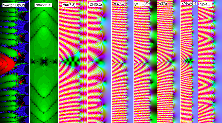
Fig 12: Left to Right: Julia sets of Newton's method on the Dirichlet L-function (5,2) and Riemann xi function, a Hurwitz zeta function and a Davenport
Heilbron function, both with off-critical zeros, two Elliptic curve
L-functions merged using a C-script to produce the echelon modular forms and
the Dedekind zeta function of the rational extension field of x4-x2-1
with central region overlayed using Computel, and a fourth degree symplectic L-function
Riemann Zeta Viewer can portray virtually any zeta or L-function
which can be represented by analytic continuation via gamma factors and Mellin
transforms, including those of number fields, elliptic curves, and modular and
Maas wave froms on hyperbolic spaces.
Parameter files for all the known examples are included with the package. The
RZ flight manual illustrates the use of a third degree Maass L-function to generate Mandelbrot and
Julia sets.
Fig 10:
Dark Heart controls portraying
![]()
Dark Heart Complex Function Viewer Flight
Manual
Dark Heart allows you to interactively explore
the fractal dynamics of a wide variety of complex polynomial, rational and
transcendental functions.
See http://dhushara.com/DarkHeart/
for research, updates and source code.
DHViewer is a matched pair application with the
Riemann Zeta Function Viewer, RZViewer, which explores the corresponding
L-functions based on Dirichlet series rather than power series.
Basics:
Drag a rectangle to enlarge a portion of the current image.
Click a point to cycle:
Function > Mandelbrot > Julia(c)*
*c at the clicked point on the
Mandelbrot set.
With keep scope on Julia view
will take you back to the previous Mandelbrot screen to save computation time
and enable you to explore several related Julia sets in the region. It will
also retain scope on a reset to function mode. To return to full screen unclick
keep scope and reset twice.
By clicking, you can investigate the discrete
dynamical parameter plane (Mandelbrot set) of the critical values and the Julia
sets of z=f(z,k,c)
for (x,y)=c,
with k an additional parameter
associated with the power.
The additional parameter k
can be set to a value other than k=2 by using Set R, I in function mode. It
generally sets the exponent but for Sin(z)/z it sets the number of critical
points. For cCos(z^k),
Cos(z^k)+c, one can set half-integer values such as
k=0.5
to get inverse quadratic cosines.
The controls all have floating help panes
to guide you.
The window can be resized to suit in real time,
resulting in a refresh and recalculation, or set to full screen using the green button. Esc to return to windowed mode.
Standard settings:
Threads enables a multi-core machine to work faster
using as many threads as coprocessors.
Max Iterations gives how many iteration steps of a point
on the Julia or Mandelbrot set before maximum iteration cutoff. Recalc refreshes and
recalculates the existing screen. Reset returns to the function
and default scale but doesn't alter any other settings. Keep scope on
click keeps the window centre and scale when clicking between
Mandelbrot, Julia and function, so the other parameters can be changed without
changing the point of view.
Menus:
About gives a complete instruction summary. Save
saves the current window's image as a tif file and all the settings for a given
calculation in a text file (see format below), enabling you to save all the
parameters for future investigation and redrawing. It will overwrite any files
of the same name. Load Parameters will load a previous
calculation and redraw it. Load Movie Seq loads a sequence text
file to generate a series of images to make a movie (see format below). Save Movie saves the
sequence as a series of LZW compressed tifs, which can then easily be
composited into a movie e.g. using open image sequence in Quicktime Player 7 (https://support.apple.com/kb/dl923?locale=en_US), or using the included app Mpeg Streamclip.
Print enables an image to be printed or exported to pdf format. Page
Setup needs to be landscape in 80% to fit the standard window on one A4
page. Help directs you to the about menu.
Advanced Settings:
Pop-up Menus: Color schemes can be changed in
real time using the color pop up menu. All the other controls require window
recalculation.
A Variety of Functions as discussed above can be explored using the
function pop-up menu.
The escape bound can be set but
resets on function change to the one most appropriate for the given function. The escape type is usually a (absolute) for polynomials and rational functions and r (real) for exponential and i (imaginary) for trigonometric functions. Setting r+ for real positive enables fine depiction of exponential Cantor bouquets, and i+ for cos and sin bouquets.
Buttons and Text Fields: Current window parameters and c values
can be read out from and written into the text fields and set by pressing the
appropriate button. Numbers in the
text fields are double precision and may appear in floating format e.g.
-7.000000186963007e-05 manifestly too large to see in their entirety in the
text box without dragging or selecting all and copying. The Julia c
values will be overwritten by the Mandelbrot critical point origin and current
Julia click point each cycle but can be manually re-entered as desired. You can use dF as a computation of the derivative of the function to locate critical points as its zeros and then when you click twice and carry it to Julia with this c
value, checking hold will keep it in the real and imag
fields so you can click SET R,I to get the Mandelbrot set to have the correct
critical point. While dF is on, you will only get the chosen
Mandelbrot set of one critical point rather than all superimposed. This enables
you to explore individual Mandelbrot sets of each critical point by inserting
it in c.
Tick boxes: There is an imaginary axis orbit trap option. Escape only tests only for escaping points. When turned off the routine also checks for attractors up to period 18, coloring internal basins, but this can also flood surrounding regions if the attractor bound is set too high for the region being investigated. When color mode is 1 instead orbit trap doubles the period search to 35 and enables adjustment of black and white shading of Siegel discs and related parabolic sets.
Sliders: Attractor
bound adjusts the size of the epsilon neighbourhood testing for fixed
point or periodic attractors. Escape bound sets the numerical bounds on points
escaping to infinity.
Color Schemes: There are several colour schemes for
function, Mandelbrot and Julia, which are useful at highlighting different
features:
Function: (0,4) rgb = logarithmic abs(z), blue cosine
abs(z), green ang(z). (1) rgb = real, imaginary and angle, (2) bg = abs(z) and
angle (3) rgb = real, imaginary and cos(angle).
Mandelbrot: (0) Sine wave colours (1) Period-coded colours that show the periodicities inside the dark hearts when Escape only is off. The escape bound slider can then be used to adjust colour shading, or to adjust velocity coded cosine in b&w for non-periodic rotations when orbit trap is selected. The attractor slider also affects hading in both cases. (2) RGB ranked colours which can also show which attracting fixed point is involved in Newton's method for k=3 and the Herman ring (3) Attractor-coded rainbow which highlights individual attractors in rational mappings, including Newton's method, by the angle, which also shows the mapping on individual sub-regions of Julia sets in terms of a rainbow in p steps where p is the period. (4) Same as (0) but with square root behavior. Very good for highlighting boundaries and complex dynamics. (5) KBCGYRM colour rotation with W. It also portrays the velocity coded cosine in b&w for non-periodic rotations with Escape only off and orbit trap is set. You can adjust the effect for different rotation rates using the escape radius slider. (6,7) Further colour schemes also used with moduli spaces.
Period
coding in mode 1 gives escaping points tending to
real infinity shades of grey from white to black in waves by iteration number
in the same way as mode 4, giving clean exteriors, with periodicities coloured approximately by the following 1 2 3 4 5 6 7 8 9 10 11 12 13 14 15 16 17 18 mildly
shaded by iteration number. You need to turn off escape only and set the attractor bound e.g to 10^-2 (default). When orbit trap is set in Mandelbrot mode, it doubles the period search to 35 colouring the higher values in lighter shades mod 18, but
this will also slow the computation. In Julia mode periods always go up to 35.
With orbit trap off you can adjust the escape bound slider
to get the right degree of color-coded shading. For periods up to 18, this
shades to black but for higher periods with lighter shades, the base colour varies. With orbit trap on both views
portray the velocity coded cosine in b&w for
non-periodic neutral rotations, as in mode 5 and gives an average colour coded view for periodic sets.
Attractor coded colours in modes 2 and particularly 3 can distinguish each basin by color
in periodic Julia sets and when there are several attractors, such as in the Newton's method
iteration. Occasionally e.g. when you set the c values of a Julia set to
0 this may give a Moire pattern anomaly, due to undeflows of the angle, which you can suppress by
choosing a neighbouring non-0 point e.g. 0.01.
Julia: (0) Sine wave colours, (1) attractor coded colours as above, (2) RGB ranked colours, (3) rainbow with potential function on escaping points. (4) As 0 but with
square root behavior. Very good for highlighting boundaries and complex
dynamics. For example the classic quadratic Seahorse Valley Julia c = -.74543 + .11301i. (5) KBCGYRM colour rotation with W as above.

Fig 10b: Variety of parameter planes using the second menu function: cz^m(1-z)^n
Functions:
You can investigate a variety of functions, [1] z^k+c, [2] cz^m(1-z)^n, [3] z^m-nz+c, [4] (z^m-n)(z+c),
[5] Int(z^m-n)(z+c), [6] z^k+(c-1)z-c, [7] Newton's method on the previous function i.e. ((k-1)z^k+c)/(kz^(k-1)+c-1),
[8] cSin(1/z), [9] cCos(z^m)^n, [10] Cos(z^k)+c, [11] c(Sin(z)+Sin(2z)/2), [12] c(Cos(z)+Cos(2z), [13] cSin(z)/z, [14] c(z^m)e^(z^n), [15] (z^k)e^z+c, [16] Transcendental (see list below), [17] Rational (see list below), [18] z^m-10qz^-p n=p.q [19] cz^(z+k), [20] c(z^3+(k-1)z^2-kz), [21] e^(-z^k)+c, [22] Quintic, [23, 24] Herman
ring function, [25] generalized Collatz iteration, [26] z^m+cz^-n k=m+in [27] cCos(z^m+z^-n), [28] Milnor rational examples
Here is a function number list mapping to the
app menu.
function number Function menu
1-3 1-3
18 4
20 5
4-15 6-17
19 18
21 19
22 20
16 21
17 22
23 on 23 on
Some of the transcendental functions are
comparable with the gamma and zeta functions in Riemann Zeta Viewer. All but a
few of the functions are unique valued on the complex plane. Although cCos(z^(1/2))
has no branch cuts, all those implicitly involving log(z), including czLog(z),
and cz^(z+k), do.
The function z^m-nz+c, can be used to
explore variations of the parameter planes as we move from z^m+c
by increasingly separating the critical points. n can be
either positive or negative, giving real or imaginary critical points in the
cases of z^3
± z.
The functions z^m-10qz^-p n=p.q and z^m-10qz^-p n=p.q (listed at the end) are accessed by inputting k=[m,p.q] e.g. for z^3-2z^-1 we input k = [3, 1.2]. You can also input negative values for p e.g. to get z^3-z^4 we input k = [3, -4.1]. Some functions might look more interesting with small values of q which bring the parameter planes into intersection.
1 (z^n)e^z+c,
You can input positive or negative values for
k into (z^k)e^z+c. The value n=0 has only the exponential plateau at x=-1000 as critical and
n=1 has this and the other critical at x=-1 as criticals so you can see the
effect of both together in mode 1. To turn off and see the Mandebrot bulbs
select dF to get only x=-1 critical.
1 c(e^z-1),
2 zLog(z)+c,
3 czLog(z),
4 z^z+c,
5 cze(-e^z),
6 z=z*e^(-e^z)+c,
7 z=(z^2-2z+2)*e^z*c,
8 z=(z^3-3z^2+6z-6)e^z*c
9 n=1..4 step triangle wave sum[j=0..n] cos((2j+1)z)/(2j+1)^2 *c
10
n=1..4 step square wave
sum[j=0..n] (-1)^n cos((2j+1)z)/(2j+1)
*c
11
-log(cos(z)*c whose derivative tan(z) has both zero and infinite criticals.
12 (tan(z)-z)*c
whose derivative (tan(z))^2
has both zero and infinite criticals
13 (z-tan(z)+((tan(z))^3)/3)*c whose derivative (tan(z))^4
has both zero and infinite criticals.
14 z-atan(z)+c
16 cze^(..n times..(e^z)) n-fold tetration (you will need to choose a critical
point using dF in function mode and then homing in on a critical point,
click to julia and select hold to insert the c into mandel mode with Set RI)
17
ce^(..n times..(e^z)) n-fold
tetration
Rational (k = (m,n))
1 z^2-1/nz*c,
2 ((z^3-1)/(z^2-1))^2+c,
3 (z^6-1)/(z^4-1)+c,
4 Int(z^3(z+1)(z^2-1))+c,
5 ((z^3-1)/(z^2-1)) ^2*c,
6 (z^n-z)*c,
7-8 Peterson graph zeta function and reciprocal (+c *c 0/1)
9 1/(z^2-c2)+c (Milnor)
10 2z^3/(27(2-z))+c (Milnor)
Rational
PrePer(2,1) Needs scale=200 Esc only off Esc Bd =10^4
11 0 1-8*(c+8)/(c-8)*(1/z-1/z^2)
Rational Period 1 mating 11 1 Per1(0) z=z^2+c
Rational
Period 2 matings 11 2, 2.5 Per2(0) z=c/z/(z+2), z=(z^2+c)/(z^2-1)
Equivalent
symmetric Julia representations
Rational
Period 3 matings. 11 3, 3.5 Per3(0) z=(z-1)(z-c/(2-c))/z/z, z=(z^2+c^3-c-1)/(z^2-c^2)
Asymmetric
and symmetric Julia reps.
Rational
Period 4 matings.
11 4, Per4(0) z=(z-c)(z-(2c-1)/(c-1))/z/z, Asymmetric.
11
4.5, 4.75 z=(z*z+((c-1)±sqrt(5*c*c-6*c+5))/2)*(1-c*c)-1)/(z*z-c*c) Double
plane symmetric Julia reps.
12 z^2+exp(2*pi*i*c)z Explores boundary of quadratic central
domain c=n e.g. n=0.618034
13 z^3-3cz+sqrt(4*c*(c+0.5)^2) Cubic Per1(0)
14 2z^3/(3c-2)-3cz^2/(3*c-2)+1 Cubic Per2(0)
15 z^3+cz^2+z*cexp(2*pi*i*n) Cubic exp(2*pi*i*n) e.g. n=0.618034
(Reset on 15)
16 (c^3-c+1)/(c^2(c-1))z^3-(c^4-c+1)/(c^2(c-1))z^2+c Cubic Per3(0)
17 (c^2-1)/(c^2)z^3-(c^3-1)/(c^2)z^2+c Cubic PrePer(2,1)
0>c>1>1
18 1/c/(c-1)(z^3-z^2)+c Cubic PrePer(1,2)
0>c>1>c
19 0,1,2,3 Cubic PrePer(2,2) 0>c>1>d>1, 4 same as 17, 5 equivalent to 18
20 0,1,2,3 Cubic Per4(0) 0>c>1>d>0, Four split parameter planes
When dF is on the particular split plane is chosen, with its Julias.
by turning on hold after the first and pressing Set R,I after each click to retain
the original location.
21 0,1 Cubic PrePer(1,3) Two split parameter planes
Per 1(0)
is cz^2(z-1)= c(z^3-z^2) (Fn 5 with k=0. Equivalent to Fn 2 with z > -z)
PrePer(1,1) 0>1>1
is cz^2(z-1) +1 (Equivalent to c(z^3-2z^2+z)= cz(z-1)^2 1>0>0, Fn 5
with k=-1, since the two iterations commute under [c,z]->[c,1-z])
Parameter
files for Per1(0), PrePer(1,1)
are included in the quintics folder.
22 c^2(2c-3)/(3-3c)*(z*z*z-z*z)+1/c Critical 0 -> 1/c -> crit 2/3.
23 c(z+0.5/z^2) Similar to Newton's example with rotational symmetry.
There
is a similar example Mandel1 in Milnor. Both use mode 3 to effect.
24 (z^2+10qc^p)/(z^2+c) n=p.q>=0,
(z^2-10qc^abs(p))/(z^2+c) n=p.q<0
E.g. (24,-3.2) is (z^2-2c^3)/(z^2+c)
25 (z^3 -10.qz ± c^p)/(z^3-10.qz+c) n=p.q as above for ±
26 (z^3 ±10.qc^p)/(z^3+c^2) n=p.q as above for ± E.g. (26,-4.1)
27 (z^q+c^p)/(z^q+c) n=p.q n<0 -> q<0 E.g. (27, 3.2) is (z^2-c^3)/(z^2+c)
28 (z^q-z+c^p)/(z^q-z+c) n=p.q n<0 -> q<0
Matings are rational function Julia sets which have
complementary components consisting of two types of quadratic Julia set fractally
intertwined. The above rational examples Perk(0) define parameter planes of
quadratic rational functions with the critical point having a fixed period but
the other one free. The Julia sets of these exemplify matings of the root Julia set of periodicity k with
the spectrum of Julia sets defined by the other critical point’s c values in the parameter plane. A broad palette of precompiled Medusa
mating parameter files are included in the matings folder which upload to the Mating function f(z)=(az^2+1-a)/ (bz^2+1-b) where a and b are input as
coefficients in the file. These allow one to use the Medusa algorithm to define
the rational function mating the Julia sets having two fractional external
angles p/q and r/s. Medusa is included
with Dark Heart, with source code, as a command line tool which can be run from
Mac Terminal by typing “./mating”. The final output of
this once convergence is reached can be portrayed in Dark Heart by entering them
into the c-script mating.c, or pasting the coefficients into one of the example parameter files. Medusa is consistent with the symmetric representations of Perk(0). If you don't have Apple's XCode installed you will need to download it, free from the Apple Store and then install the Terminal command line tools by executing xcode-select --install in Terminal to activate gcc. On older systems, a suitable version of XCode can be downloaded by signing on for a free Apple Developer account. The script can also be edited, compiled and run in XCode as a command line tool
By saving and adjusting the coefficients and powers of c in the test file, and reloading, you can portray parameter planes and Julia sets of any polynomial up to degree 5. The application will automatically find the critical points up to degree five. The application comes preprogrammed with a sample quintic f(x)=x^5-3.25cx^3+2.25x+c to illustrate how to program different parameter planes. This will be overwritten on loading a saved parameter file. You can use this to replicate several parametrizations e.g. z^4+(c-1)z-c can be cloned as z^4-sz-1+s, s=1-c. See parameter file contents below for details.
Newton's method on the k-th roots of unity shows how seeking for the roots of a function by iteration can leave behind a chaotic boundary set where the iteration can’t reach the attracting roots. To see the standard Julia set of the roots of unity, insert the value (0,1) into Julia mode, since c = 1 gives z^k+(c-1)z-c = z^k-1. If this is run in attractor coded modes 3 (or 2) the basins are individually colour coded. For k = 3 in RZ 2.0.6 you can set the imaginary part to -1 to get the repelling version. Higher powers don't work here because the forward Newton’s method has critical points determined by z=0 and the c-displaced roots of unity, since the derivative of g(z)=z-f(z)/f '(z) is g'(z)=f(z)f ''(z)/(f '(z))^2, and the super-attracting displaced roots have infinite parameter planes and can be ignored, but the inverse repelling process gives g'(z)=2- f(z)f ''(z)/(f '(z))^2, whose 2k-2 degree equation can be solved only for k ≤ 3. This dynamic is almost entirely repelling except for Julia kernels determined by the small isolated Mandelbrot islands.
The Herman ring in cz^2(z-4)/(4z-1) is a famous special rational function case with an
irrational annular flow for Julia sets for which c= exp(i*g*pi/2) = 0.564635 +
0.825341i, or c= exp(i*g*pi)= -0.3624 + 0.9320i where g = (5^(1/2)-1)/2 the
Golden Mean. Choose colour mode
5 and have escape only turned off and input the precise numbers into
Set R/I and you can see the rotation pictured in cosine of the velocity. You
can adjust the effect for different rotation rates using the escape bound
slider.
You can view the Herman ring system in two
configurations, making Mandelbrot sets for each of the two parametrizations cz^2(z-k)/(1-kz)
and kz^2(z-c)/(1-cz). If you switch from the second
function to the first just before clicking a point in Mandelbrot mode it will
retain Mandelbrot mode, save c as k, and allow you to input the second
parameter c by clicking. You can see the k=m,n values in Set R, I in function
view. A further click takes you to the k, c Julia set.
Similarly to the Herman ring, the standard
quadratic function z^2+c has Julia
sets with irrational flows on Siegel discs between all the fractal bulbs on its boundary for
example at c = -0.390541-0.586788i , which is a solution of the cardioid c=exp(ig2pi)/2-exp(ig4pi)/4
for g = (5^(1/2)-1)/2. You can contrast this with the period 3 parabolic petals
on the boundary of the cardioid c=-0.125000-0.649519i which clearly shows it is
in transition between period 1 and 3 at 1024 in mode 1. The 20 leaf parabolic
Julia set c = .27334 + .00742i shows its leaves on mode 5 with escape bound
10^3 at 4096 iterations.
A
series of C-script examples of rational parameter planes are also provided
under the Milnor function option which explores the iterations z > 1/c(z+r.c+s+1/z)
and its dual z > r/(c-s)(z+c+s +1/z).
One
can use z^m-nz+c, and (z^m-n)(z+c) in modes 3, 6 or 7 with orbit
trap selected to explore moduli spaces of these Mandelbrot sets, as they
have dihedral symmetries. Two c-values c1 and c2 of such functions are
conjugate under a Mobius transformation f(z)=(az+b)/(cz+d)
if and only if c2=w*c1 with w an p-th root
of 1 (p=m-1 in the former case) where the symmetry is by an p-th
of a revolution. Hence we can take equivalence classes of such c to form
a new complex plane C=c^(1/p), displaying each equivalence
class and its conjugate, which fully classifies the resulting Julia sets up to
rotations by 2*pi/p.
One
can also use z^m-nz+c,to explore the Mandelbar equivalents conj(z)^k-nz+c , by inputting k=(m+100,n) for m a positive integer
≥ 2. The classic Mandelbar is conj(z)^2+c , which you will get by setting k=(102,0).
The Collatz system gives you the complex
generalization of the 3n+1 problem n -> n/2 if n
is even or n -> 3n+1 if n is odd (or (3n+1)/2 for k=2,
since this saves one step. This is generalized to (cz+1) (k=1 for
c=5,7,9)
(z/2)Cos^2(piz/2)+((cz+1)/2)Sin^2(piz/2)
and shows why although all positive integers in
the 3n+1 problem eventually end up in the 3-cycle 4>2>1 for
complex values we have fractal chaos.
Set k using function view and
then c using Julia view. (k,c) = (1,3) and (2,3) give the
standard and reduced Collatz sequences as above. You can also set 5n+1
and 7n+1, which give both periodic and chaotic escape to infinity for
given values.
You can use color mode 1 to check the periods
of the Collatz (3n+1 n odd n/2 n even)
iteration. Set up the Julia iteration as above, and set color 1 with escape
only off and attractor bound 10^-2 (default) with Max
iterations set to 1024. Then set RIS for (x=n,y=0) and
use scale to zoom in. For positive integers you get period (3),
for -1 (2), -5 (5) and -17 (18).
You can also check 5n+1 e.g. 4, 6 give period (7), 5
gives (10), 7, 9 give (chaos) and -4
gives (3). 7n+1 gives
either period (4) or (chaos).
The function z^m+cz^-n gives symmetrical
Mandelbrot sets with unique Julia sets of three types, Cantor set (Fatou dust)
of points, Cantor rings (simple closed curves) and Sierpinski curves (fractal
Swiss cheese). The function and Julia sets have m+n-fold
rotational symmetry while the Mandelbrot set has (n-1)-fold symmetry,
despite there being n+m free critical points.
The final function is the zeta function of the
Petersen graph, a degree-24 polynomial with multiple critical values, giving
high order Julia sets. The parametrizations of both cPetersen
and Petersen+c are given for comparison (k=0 inverse +c k=1 inverse *c k=2 original +c k=3 original *c ). You need to have escape only turned off for the last two.
You can investigate the Rieman Zeta function
and a variety of other zeta and L-functions using Riemann Zeta Viewer which is
designed to deal with these advanced functions.
Parameters Text file format:
[0] mandel (2=function, 1= Mandelbrot, 0=Julia), [1-5] Scale, X, Y, (Fn k J/M c) R, I, [6] the current function, [7] escape type (abs real or imag), [8] orbit trap (0/1) + 2*dF + 4*mval (0=use std crits / 1=use input crit), [9] escape only (0 or 1), [10] color scheme (0 to 3), [11] escape bound (exponent 10^n), [12] attractor radius epsilon bound (negative exponent 10^n), [13] maximum iterations, [14-15] real and imaginary values of k, [16] previous function [17] dummy 987.654321 so you can find >> [18-29] complex coefficients a + bi of a polynomial up to degree 5 (6 pairs of
reals), [30-35] powers of c (usually 0 or 1) multiplied into each
coefficient of the polynomial for the Mandelbrot plane. [36] Additive c.
Two C-scripts are provided to explore polynomials. The C-script crits.c will generate any polynomial up to degree 5 from its critical points, scaling and rotating these together as required, enabling one to generate examples with arbitrary criticals in a given position. The script coefs.c provides an easy way of setting up an arbitrary polynomial up to degree 5 from its coefficients and parameter plane c values. See additional software for scripts below.
Movie Sequence Formats: The text file consists of series of floating point numbers. (1) File format 1-3 (2) N<=1000 number of frames (3) 1/0 Mandelbrot/Julia followed by a sequence of frame parameters [ X, Y, Scale CX, CY]. Format 1: only the start and end parameters are specified and DHViewer will generate N frames in a linear sequence between these values. Format 2: the file supplies a series of N parameters on any trajectory, for instance computed values running around the cardioid of a Mandelbrot set. Format 1 and 2 files can either generate blowups of Mandelbrot sets or movies of Julia sets as CX and CY vary. The sequence file has no parameters except mandel, so you can set all the other settings manually before saving the movie. If you want to determine in advance the complete parameters for a movie run, save your parameters and load them before loading the movie sequence file. Format 3: The format file contains only parameters 1 & 2 and is accompanied by a series of full parameter files, generated by another application such as the C-scripts attached which can be run from Terminal. If the format file is myfile.txt, the parameter files need to be numbered myfile0.txt - myfileN,txt. This format enables batch programming of any sequence of images automatically.
The file moduli8.c illustrates an extreme geometric scaling blowup using scientific notation fprintf("%e") rather than the 6 decimal point precision of fprintf("%f"), which can be used in any of the other c-scripts as well.
Ultra-large images: The file 'large.c' in the rational folder enables the generation of very large Julia and Mandelbrot images suitable for poster size displays. The script can be adjusted to generate a set of tiles in the standard window size of 750x513 using a set of image parameters you have saved as a parameter file. A file 'page.png' is also included in the folder, which forms a white background 7500x5130, which can be opened in Preview. You can then paste each of the tiles into the large page to get an expanded size image, by choosing actual size and pasting and lining them up carefully. An app to do this automatically is in development..
A series of movie scripts to generate the movies of the cubic separations is included with a manual of how it was created to give an example of using Dark Heart to generate trajectory variations in the field of view as satellite Mandelbrots or Julia parameters change in non-linear ways. The file moduli8.c illustrates an extreme geometric scaling blowup using scientific notation fprintf("%e") rather than the 6 decimal point precision of fprintf("%f"), which can be used in any of the other c-scripts as well.
Associated Files
Along with DHViewer are sample projects to show
file handling:
1. Load Parameters for z^5-z^4+z^3-cz^2+z-c to
see an example of a Mandelbrot plane of an arbitrary 5th degree polynomial
2. To generate a movie sequence sample:
(a) Load Parameters for z^3-z+c.txt
(b) Load Movie Seq cubic.txt
(c) Save Movie to an empty folder get a 500 frame Julia movie sequence.
3. To generate an 8 frame sample movie using
Format 3:
(a) load test.txt
(b) Save Movie to an empty folder to get an 8 frame evolution of
cz^(z+k) defined by parameter files
test0.txt-test8.txt
4. Four template movie sequence files are
included in movie C-scripts. You can run the sample files from Terminal as
shown in each file header. This is a fully programmable interface which
provides a template for much more powerful movie making.
Additional Software for
Scripts and Movies
Movie frames are in tiff images which can be turned into Quicktime movies with Quicktime Player pros 7's open image sequence option, or using Mpeg Steram clip, which is included with the package. If terminal doesn’t recognize the gcc command, open an Apple Developer account (free) and install Mac OSX Command Line Tools for your system from https://developer.apple.com/download/more/
Fig 11: Rieman Zeta Viewer
controls portraying a degree-3 Maass form L-function.
Riemann Zeta and L-function Viewer Flight
Manual
Riemann Zeta Viewer allows you to interactively explore the complex Riemann zeta function:
Zt(z)=Sum[1,∞](1/nz)=Xct[p prime](1/(1-p-z))
a host of its Dirichlet L-function
variants and their transformations and those of a diverse spectrum of abstract
zeta and L-functions as well, right to the cutting edge of mathematical
science.
RZ operates in the same way as Dark Heart
viewer, but has some additional controls, so we will go through the manual from
scratch for completeness.
By clicking, you can investigate the Mandelbrot
set of these functions for a variety of critical values, and the Julia sets
of z=f(z)+c (or z=cf(z)) for (x,y)=c.
You can also investigate related functions eta,
xi, the derivatives of each function and Newton's method (see below).
By uploading the provided parameter files you
can also investigate abstract L-functions of elliptic curves, extension
fields and modular forms and/or generate movies of the
dynamics.
Basics:
Drag a rectangle to enlarge a portion of the current image.
Click a point to cycle:
Function > Mandelbrot > Julia(c)
at the clicked point c on the Mandelbrot
set.
Clicking the Julia with keep scope
on will take you back to the previous Mandelbrot screen to save computation
time and enable you to explore several related Julia sets.
The controls all have floating help panes
to guide you.
The window can be resized to suit in real time,
resulting in a refresh and recalculation, or set to full screen using the green button. Esc to return to windowed mode.
Standard settings:
Threads enables a ual, or multi-core machine to work
faster using as many threads as coprocessors. Max Iterations gives how many iteration steps
of a point on the Julia or Mandelbrot set before maximum iteration cutoff. Recalc refreshes and
recalculates the existing screen. Reset returns to function view.
Keep scope keeps the window centre and scale when clicking
between Mandelbrot, Julia and function, so the other parameters can be changed
without changing the point of view. A double Reset with keep
scope off returns to the default scale on the second click. To Reset
to other functions after loading an abstract L-function, you will first
need to renter a suitable L(m,n) such as (1,1) for zeta, as the value of m has
been set to 0 to override these settings with the loaded coefficients.
To facilitate locating critical points for
calculating Mandelbrot sets, tick dZ and explore the derivative
function for a critical point (a zero of the derivative looking like a dimple).
Use dragging to blow up to high resolution. Tick Keep scope and
slowly click twice right on the zero without moving the mouse. The c-values
will now appear in the Julia portrait. Then tick Hold, untick dZ
and click twice through the original function to the Mandelbrot set. The c-values
are retained in the text field by Hold. Now untick Hold and click
the Set R,I button
and you will get the Mandelbrot sets of the given c-value.
To facilitate fast fractal iteration, the
default is 100 function series terms and a cutoff of 64 iterations for each
point of the Mandelbrot and Julia sets, but these can be adjusted for greater
accuracy.
Menus:
About gives a complete instruction summary. Save
saves the current window's image as a tif file and all the settings for a given
calculation in a text file (see format below), enabling you to save all the
parameters for future investigation and redrawing. It will overwrite any files
of the same name. Load Parameters will load a previous
calculation and redraw it. Load Movie Seq loads a sequence text
file to generate a series of images to make a movie (see format below). Load Bitmap loads a bitmap
of values of a function generated by another application. Computel and Sage
scripts are included (see below). Save Movie saves the sequence
as a series of LZW compressed tifs, which can then easily be composited into a
movie e.g. using open image sequence in Quicktime Player 7 (Download: https://support.apple.com/kb/dl923?locale=en_US), or using the included app Mpeg Streamclip.
Save Bitmap saves a bitmap of complex function values for
subsequent math processing if the image has previously been refreshed in colour
scheme 5, which also produces a useable bitmap in its tif files. This is to
keep the other colour modes as fast as possible. The bitmap saves the values of
the function, so doesn't care about the colour scheme. Print
enables an image to be printed or exported to pdf format. Page Setup
needs to be landscape in 80% to fit the standard window on one A4 page. Help
directs you to the about menu.
Advanced settings:
Pop-up Menus: Color schemes can be changed in
real time using the color pop up menu. All the other controls require window
recalculation.
Functions related to zeta, including eta, xi, gamma, psi
and others discussed below can also be explored using the function pop-up menu.
For completeness, an alternative Gamma product formula, can be used
instead of the default Lancos approximation, by pulling down the pop-up menu to
choose a power of 10 terms in the product, but is slower and less accurate
unless 10,000 iterations are used.
Buttons and Text Fields: A function terms text field is
provided to set how many terms are calculated in the chosen sum or product
function, with a default of 100 for speed of initial exploration. This can be
adjusted to exact large values which have anomalous behavior (see end). Current
window parameters and c values can be read out from
and written into the text fields and set by pressing the appropriate
button. L(m,n) text
fields enable examining a wide variety of Dirichlet L-functions as well as Zeta
and Eta. Numbers in the real text fields are double precision and may appear in
floating format e.g. -7.000000186963007e-05 manifestly too large to see in
their entirety in the text box without dragging or selecting all and copying.
The Julia c values will be overwritten by the Mandelbrot critical point
origin and current Julia click point each cycle but can be manually re-entered
as desired.
Tick boxes: dZ finds the approximate formal derivative
of any function being displayed. Good for finding critical points since these
are the zeros of the derivative. It works only in function mode. For fractals
use dZeta or dXi. You cand get the second derivative approxiation by combining
the two. Full Terms is located on the pain page as a control and
as an attribute. It forces the current function to use all the specified series
terms. Otherwise it breaks off if the terms get smaller than 0.001 the size of
the sum. Occasionally not having Full causes strip dislocations in a few
regions. The control has immediate effect during drawing and is useful if a
slow blow up of a Julia set needs to have full iterations just for the complex
boundaries of the kernel. Mellin
uses a Mellin transform in the central region if the function admits an analytic
continuation. Like Full Terms, it is active during drawing. The logFn.
tick box examines the log of the selected function. Split sets
the functional equation split (-1 > -100, 0>0, 1>0.25, 2>0.5). Xi
calculates the xi function instead of zeta/L. R- escape makes the escape path negative only highlighting the Cantor bouquet structure. Mobius transforms the complex plane, mapping
the line x=1/2 onto the unit circle, so you can see the whole extent of
the Dirichlet functions. For the exact mapping see below. Escape only
tests only for escaping points, to avoid spurious periodic solutions from
overwriting escaping orbits, but is slower because attracting orbits have to
run to the Max interations for each point. The application defaults to this being off and colours most
modes so escape to the right is colored the same as non-escape speeding the
calculations, but to get high resolution images of small Mandelbrot and Julia
kernels you may need to turn it on. crVal uses critical value
instead of critical point for Mandelbrots. This is useful for generating
parametric movies running between critical values. See blue skies method below
for finding critical values. The tick box +c/xc changes the
parametrization from f(z)+c to cf(z) giving
a second parameter plane and collection of Julia sets for each function. Angle
turns on and off the green/yellow display of the angle (argument) of f(z)
in function view for each mode. Rotate rotates the image by pi/2
to assist viewing the critical line.
Sliders: Attractor
bound adjusts the size of the epsilon neighbourhood testing for fixed
point or periodic attractors. Escape bound sets the real absolute bounds on points
escaping to infinity.
Colour Schemes: There are several colour schemes for
function, Mandelbrot and Julia:
Function: (0) Absolute-Angle mode rgb =
red logarithmic abs(z), blue cosine abs(z), green angle(z). This is the most
informative although not the most appealing (1) Real-Imaginary mode
rgb = real, imaginary and angle, (2) X-ray mode with red, cyan
real~0 and imag~0, by exp(-x^2), adjustable by the attractor bound, overlaying
bg = abs(z) and angle(z)
Highlights gram points with real=0 on x=1/2 and zeros at the
intersections of real~0 and imag~0. (3) Positive-Negative mode.
Highlights the positive and negative real (r~c), imaginary (g~m) and angle by
1-cos (b~y). (4) Log-angle mode This method uses abs(log(1/(1-Z(z)))
for the absolute value, adjustable using the escape bound slider, retaining the
angle of Z(z). This still highlights the zeros since
log(1/(1-0))=log(1)=0 but highlights variations in the function to the right of
the critical line. It is good at highlighting the function in the right
half-plane and in the crtical strip in a way which evenly compares asymptotically
large and near-unitary values. (5) Soft mode rgb = cos(angle) sin(angle),
abs(z). Good for retrieving function data fromthe tif file.
Mandelbrot: (0,5) Sine wave colours, (1) Attactor coded
colours, giving escaping points tending to real infinity shades of grey from
white to black in waves by iteration number with periodicities coloured
approximately by the following 1 2 3 4 5 6 7 8 9 10 11 12 13 14 15 16 17 18 mildly shaded by iteration number. You need
to turn off escape only and set the attractor bound to 10^-2
(default). (2) RGB ranked colours (3) Potential function rainbow. (4) attractor coded inverse quadratic.
(Highlights geometrical details lost in high iteration numbers). (5) Attractor
coding giving escaping points tending to real infinity green through orange and
points remaining finite coloured by decreasing blue by iteration, combined with
redness corresponding to the attractor period. When R- escape is set in mode 1 it doubles
the period search to 35 colouring the higher values in lighter shades mod 18,
but this will also slow the computation.
The 'critical' point for the Mandelbrot set is
chosen to represent a prominent critical landmark. For zeta, eta, mu, and sigma
it is chosen to be 1000 corresponding to the limit f(z)>1 as
real(z)>+∞. For gamma it is 1.465. For Xi it is 0+ki, k=0.00000001~0.
Other critical points can be chosen using the advanced settings and inputing CX
CY values under Mandelbrot mode, just as c values can be inserted for any Julia
set. A list of critical points for zeta eta and xi is provided below, or can be
approximated using the values of
observed zeros of dzeta etc. You can also input CX and CY in function mode to
generate a transform of the function, whose zeros are at the fixed points of
the critical values [f(cv)-v=0 or f(c+v)-v=0] and hence candidates for being in
Mandelbrot kernels of the critical points.
You can flip easily between Mandelbrot mode and
transformed function mode using 'keep scope on click'. To exit reset. This can
potentially find a finite number, out of the infinite collection of kernels,
but sometimes the one located is vanishingly small, leading to blowing the
mantissa of the floationg point doubles before we reach it.
Not all the functions have meaningful
Mandelbrot sets. The zeta attracting fixed point is at -0.2959050055752.
Julia: (0) Sine wave colours, (1) Attractor coded
colours, (2) RGB ranked colours, (3) Rainbow with potential function on
escaping points. Colour coded Julia attractors have blue shaded to escaping real, red shaded to periodic
attractor, green non-negative periodic attractor, with grey indeterminate. The
red and green are tinged with blue to indicate the period. (4) Attractor coded inverse
quadratic. (5) Attractor coded with RGB mapping.
For exploring the higher zeros of zeta, a high
number of series terms can be set using the slider. Values of the RZ function
outside the critical strip [0,1] are set to 0 after y=±450i because the sin/cos
component of the analytic continuation overflows to Inf. This leaves the zeros
in the critical strip still well rendered up to values in the millions with the
highest number of zeta iterations set in the slider.
The Functions:
The package is designed to facilitate research
into the widest spectrum of zeta-related and L-functions possible. Each of zeta, eta and all the
L-function variants L(m,n) for m up to 63 are
encoded as a generalized zeta function which can then be differentiated, or
have any of the functions from xi, through those like lambda and mu whose
coefficients are important arithmetic functions, to the Newtons method's and
differentiation applied to them. This creates a widest a diversity of
exploratory functions as possible.
Zeta
Zt(z)=Sum[1,∞](1/nz)=Xct[p prime](1/(1-p-z))
Zeta is represented here in terms of Eta as:
Zt(z)=E(z)
/(1-21-z) for real(z)≥0
and by analytic continuation using:
Zt(z)=2((2pi)z-1)cos(pi(1-z)/2)G(1-z)Zt(1-z) for real(z)<0.
http://en.wikipedia.org/wiki/Riemann_zeta_function
Eta E(z)=Sum[1,∞]((-1)n/nz)
E(z)=(1-21-z)Zt(z)
Used to extend Zeta from real(z)>=1
down to real(z)>=0.
To access it set L(m,n)=(1,-1).
http://en.wikipedia.org/wiki/Dirichlet_eta_function
Dirichlet L-functions
DL(z)=Sum[1,∞](X(p,q)/nz)
where X(p,q) is the qth set of Dirichlet
characters of period p.
Enter p=Xm and q=Xn into the L(p,q) text
field. Each of the other variant
zeta functions can be applied to any of the L-functions as well as zeta and
eta. The viewer calculates the finite residue groups Z/Zn
generating the characters, factors both for sub-periodicities and for
conductors, and then applies the correct functional equation and prime
multiplicative factors to give the full representation on the complex plane. A
Mellin transfor is performed in the central basin to improve fidelity.
A Terminal C-script is included with the
application files which shows how a given character cast X(m,n) is generated and reduced to its
primitive form. If you don't have Apple's XCode installed you will need to download it, free from the Apple Store and then install the Terminal command line tools by executing xcode-select --install in Terminal to activate gcc. On older systems, a suitable version of XCode can be downloaded by signing on for a free Apple Developer account. The script can also be edited, compiled and run in XCode as a command line tool..
Abstract zeta and L-functions
Examples such as those of elliptic curves, number fields and
modular forms can be uploaded by including their coefficients and functional
equation parameters in the appropriate file format and viewing as raw/abstract.
A suite of preloadble cases is provided in the
files along with the Terminal C-scripts which generated them and Computel PARI-GP
and Sage scripts which generated the Dirichlet series coefficients. Some of the
examples (particularly the field extensions) display convergence problems in
their critical strip similar to naked Riemann zeta , requiring a Mellin
transform treatment as is done for Dedekind/Hecke functions, but many of the
elliptic curve and the modular form examples give quite accurate portraits. A
working copy of PARI-Computel is included with RZViewer, so all the examples,
except for the modular form coefficients, can be generated without use of Sage.
Gamma G(z) the compex number extension of integer
factorial n!
By default, the Lanczos approximation is used:
http://en.wikipedia.org/wiki/Lanczos_approximation
or alternatively the product formula
G(z)=Xct[(1+1/n)z /(1+z/n)]
with n=10^k terms if alt gamma
is set to a non zero value.
http://en.wikipedia.org/wiki/Gamma_function
Xi/xi X(z) = (z-1)G(z/2+1)pi-z/2Zt(z)
This is now included for every function
possessing a functional equation,
including abstract L-functions, by
selecting in the Xi tickbox.
The unction provides a symmetrical presentation
of the zeros on x=1/2.
http://en.wikipedia.org/wiki/Xi_function
The xi functions of Dirichlet L-functions are
also included, as well as the
equivalent singularity bearing Xi function of
zeta for Xm=1 Xn=0.
Note: Xi is rotated so the zeros are on the critical
line, rather than the real axis.
The following set of derived zeta functions all
work also for any L-function.
Mu M(z)=Sum[1,∞](mu(n)/nz)
M(z)=(1/Zt(z))
The Möbius function mu(n)
= (-1)^k when n has k
distinct prime factors of multiplicity 1, and 0 otherwise.
http://en.wikipedia.org/wiki/Möbius_function
Sigma S(z)=Sum[1,∞](dvs(n)/nz)
S(z)=Zt(z-1)Zt(z)
The divisor function dvs(n)=
Sum(d : d | n).
S[k](z)=Zt(z-k)Zt(z)
gives dvs{k](n)=Sum(d^k : d|n).
http://en.wikipedia.org/wiki/Divisor_function
Lambda L(z)=Sum[1,∞](Lam(n)/nz)
L(z)=(-Zt '(z)/Zt(z))
The Mangoldt function Lam(n)
= log(p), n=p^k and 0 otherwise.
http://en.wikipedia.org/wiki/Mangoldt_function
lambda l(z)=Sum[1,∞](Lio(n)/nz) = Xct[p prime](1/(1+p-z))
l(z)=Zt(2z)/Zt(z)
The Liouville function lam(n)
= (-1)^om(n), om(n)=no. of prime factors of n counted with
multiplicity.
http://en.wikipedia.org/wiki/Liouville_function
Phi H(z)=Sum[1,∞](tot(n)/nz)
H(z)=(Zt(z-1)/Zt(z))
The totient function tot(n) =
no.of positive integers k ≤ n coprime to n.
http://en.wikipedia.org/wiki/Totient_function
dGamma, dXi and dZeta are the
derivatives G'(z), X'(z) and Zt '(z)
or any of the L-functions in zeta with xm and xn set. You can also perform an
approximate formal derivative of any function at all using the dZ tick box to loo for critical points to
source Mandelbrot sets, but this is active only in function mode. To see
fractals of the derivative function use dZeta. You can also view the second derivative of a function,
but not its fractals by combinining both.
NewtonZ, RepellngNZ and NewtonX are the Newton's method functions for
zeta, and xi.
NZ(z)=z-Zt(z)/Zt '(z), NZ(z)=z+Zt(z)/Zt '(z)
They are provided because they naturally relate
to the zeros.
zZeta is included to demonstrate the periodicities
in the multiplicative parameter plane
zetaprod is the product version of zeta or any L-function
Xct[p prime](1/(1-X(m,n)p-z)), which is technically defined only for real(z)>1,
included for comparison with zeta the analytic continuation version above. Zetaterms adjusts the product terms in
the same way as with zeta.
primeZeta is the function
Zp(z)=Sum[p
prime](1/pz)=Sum[1,∞] (mu(k)/k)log(Z(kz))
where mu is the Möbius function (see above). It
is included for completeness. It is defined only for real(z)>0.
Dedekind/Hekke L(m) Explores the Dedekind zeta and Hekke L-functions
of the field extnsion of Q to include the Gaussian integers Z[i]
= {a+ib) a,b, in Z}
L(z,l)=Sum[(m,n)≠(0,0)
∞]X(m+in)/(4(m^2+n^2))=Xct(1/(1-X(p)/(4(m^2+n^2)))
X(a)=(a/conj(a))^l
Enter l into Xm. Xn has no
effect. These functions have a Mellin integral transform in the critical
strip 0 < x < 1, for
small y for |Xm | <10.
abstract/raw zeta/L is a direct computation of Sum[1,∞](X(m,n)/nz).
Used from saved parameter files it can also be
used to generate abstract
zeta and L-functions, including those of
elliptic curves and modular forms with varying functional equations and gamma
factors. See the section on uploading parameter files and the installation file
set for examples of each.
Davenport consists of a finite collection of zeta
functions which have a similar functional equation, but (5,1), (5,2) and (7,1)
have no Euler product. (5,1) is the Davenport-Heilbronn zeta function which has
occasional zeros off the critical line, e.g. at .808517 + 85.699348i,
.650830 + 114.163343i, .574356 + 166.479306i, .724258
+ 176.702461i. (5,2) and (7,1) also have interesting off line
zeros. The remainder: (2,1), (2,2), (3,1), (3,2), (3,3), (4,1), (4,2), (6,1),
(6,2) and (8,1) are derived functions of Riemann zeta and Dirichlet L-functions.
In addition (1,n) gives (5,4)*n/1000+(5,5)*(1-n/1000) a linear combination of two zeta/L-functions with
the same functional equation with zeros off-critical. (9,th) gives a functional combination
{0,1,tan(th),-tan(th),-1}=(sec(th))/2[DL(5,4)e^(-i
th)+DL(5,2)e^(i th)]
which equals (5,1) at th=100 and (5,2) at
th= -468. [-pi pi] = [-567 567].
As this function writes and reads DL
information from memory, threads are set to 1. A
gif file of the definitions of these functions is in the attached files.
theta is the Riemann-Siegal theta function
Th(z)=log(G((1+2zi)/4)-log(G((1-2zi)/4)-zlog(pi)/2
RSZ is
the Riemann-Siegal Z function
Z(z)=exp(i theta(z))Zt(1/2+iz)
Hurwitz zeta functions H(z,a)=Sum[1,∞](1/((n+a)z) generalize Riemann zeta.
Xm, Xn provide a=Xn/Xm, (Xm,Xn)=1
Xn<Xm. These also have unreal zeros off the critical line. H(z,1)=Zt(z),
H(z,1/2)=(2^z-1)Zt(z),
H(z,p/q)= (q^z)Sum[1,q](conj(X(p))DL(q,p))
As this writes and reads DL information from
memory, threads are set to 1.
zeta-z enables one to explore the behavior of the
atrtracting fixed point of zeta
pi^(-z/2)*zeta gives a function demonstrating all zeros are
simple of first order as Z(z)=pi^(z/2)Prod[1-z/r]/(2(z-1)Gamma(1+z/2)),
r non triv 0
Psi (Digamma) P(z)=G'(z)/G(z) the logarithmic derivative
of gamma
http://en.wikipedia.org/wiki/Digamma_function
Bitmap imported bitmap to display (see below)
Power Series gives the power series
P(z)=Sum[1,∞](a(n)z^n)
corresponding to the Dirichlet series L(z)=Sum[1,∞](a(n)/n^z) either
of character Xm, Xn or uploaded as a coefficient set (see below).
Fourier does the Fourier series viz F(z)=Sum[1,∞](a(n)exp(2pinz)) either of character Xm, Xn or
uploaded as a coefficient set (see below).
Both the two above functions are useful when
examining modular forms which are expressed as Fourier series in the upper
half-plane or as power series in the unit circle. By selectng Escape Only,
you can set the areas where the functions are formally undefined to black. By
also selecting R- escape, you add 1 to the result which enables loading an
Eisenstein series leaving out its leading 1 in the same way as an L-function so
that one can do a Fourier or Taylor portrait of all the components of a modular
form space.
1/(k^z) and 1/(1-k^-z) etc. give sum and
product component functions input by k=function terms.
Weierstrass plots a Weierstrass modular function using the
first two complex coefficients of any Dirichlet or loaded abstract L-function
as periodic vectors w1 and w2 on a parallelogrammatic grid extending for
2*sqrt(fnterms) to illustrate what modular functions associated with elliptic
curves look like.
zetaFact
If Ln = 1 F(z)=Sum[1,∞](Facts(n)/nz) = Xct[2,∞] (1/(1-n-z))
Facts(n)= number of unordered
factorizations of n.
If Ln = -1 F(z)=Sum[1,∞]((-1)^Facts(n)*Facts(n)/nz)
otherwise F(z)=Sum[1,∞]((-1)^n*Facts(n)/nz)
This gives an example of a function with a
product that doesn't involve primes. It is included as a script file example
with the application files.
Theta and RSZ have been rotated so that the
zeros are on the critical line rather than the real axis. The chequerboard
effect is an artifact of the log when the gamma function rotates through the
principle value as the imaginary part of z increases. A clearer view of
RSZ is gained by turning off angle.
Mobius transformation: M(z)=(a*z+b)/(c*z+d) k=40.0, a=k+1/2, b=1-a c=d=1; with inverse M'(z)=(d*z-b)/(-c*z+a). This takes -1 to infinity, 1 to 1/2 and i to 1/2+40i, thus wrapping the critical line around the unit circle. In our case the inverse transformation is M'(z)=(x+39.5)/(z+40.5), so 0.9753 = 39.5/40.5 maps correctly to 0 to give the Julia set of zeta.
Parameters Text file format:
[0] Mandel (=2 function =1 Mandelbrot =0 Julia), [1-5] Scale, X, Y, cr,
ci, [6] altgamma (0 or 2-4), [7] the current function, [8] theoretical dzeta
(0, 1, -1 2), [9] R- escape, [10] addtive or
multiplicative c [11] escape only (0 or 1), [12] color scheme (0 to 3), [13]
escape bound (10-100), [14] number of zeta terms, [15] attractor radius epsilon
bound, [16] maximum iterations, [17] do log of fn [18] angle included in colour
scheme [19] Mobius [20] cval (holds entered critical point), [21] old fn. [22]
real k [23] imag k [24] crval+2*Xi [25] full terms+2*dZ+4*Mellin [26] xm [27]
xn [28] flip.
Arbitary Dirichlet series: You can also add additional parameters to a
saved text file or scripted movie file to define an arbitrary generalized Dirichlet series Sum[an]*[n+bn]^-z
of up to 1024 terms. These are not saved, as they cannot be adjusted in the
advanced settings. xm needs
to be set to 0 and xn to 2 to cause the system not to override k
and h. [29] character period length k, [30] chr. type h (2 or -999 or
-998). Type 2 has k real and imaginary coefficients which can be varied
in a movie script. Type -999 has both k coefficients a(n)
and an additional k adjustments n+b(n) to the
integers n forming the powers n^-z. In this way we can generate continuous
movies which pass between L-functions, using non integer exponent bases. Type -998 is used to instead
multiply the resulting function with integer coefficients by (1-2^(1-z))^-1
to convert an eta type series into its zeta form.
Abstract L-functions:
you can upload an abstract zeta/L function using the character period
length k [29] with Dirichlet
series coefficients as above with chr. type h = -997, appended after the
k complex coefficients by adding the following values also as complex
coefficients: d=number of gamma factors g((z+k1)/2),
g((z+kd)/2), k followed by k1, ... kd, N
the conductor, e the sign of the functional equation, and finally w
the weight. h = -995 has the same parameters entered as complex numbers
to allow for Dirichlet and Mass L-series with complex gamma factors
and e terms. For L-functions with very
rapidly growing coefficients which would cause numerical overflow (large
weights) enter chr. no -996, scale down the coefficients of n by a factor
n^(-sh) and enter sh as a shift factor after the weight. If you set an e
with absolute value d other than 1 you will get d ^(-z)*L(z)
which is useful for generating the full set of modular old forms (see my
research article at the web site). If the imaginary part of the weight is set
to 1 rather than 0 the powers of pi in the functional equation will be
translated by the gamma factors or their conjugates.
You can explore abstract L-function
fractal sets, save an image and parameter file. You can then load the
parameters for the image later after making sure you have first loaded the
correct L-function and the existing abstract function will continue to
operate.
If the abstract L-function has 2 gamma factors
of 0 and 1 respectively and Mellin is set, RZViewer will also use the Mellin
transform for a modular form (or elliptic curve) in the region 0≤x≤w, -8≤y≤8 to
improve fidelity in the central basin. This is useful for considering the Birch
and Swinnerton-Dyer conjecture. Finally with version 1.7.3 a general Dokchitser
type gamma function inverse Mellin transform routine has been instituted for arbitary
L-functions which is currently experimental, but works successfully on the
genus 2 and 3 examples. To activate this fullterms needs to be set to 4 in the
parameter file. In both the modular and general cases, if the number of gamma
factors is given a negative sign, the three terms after weight (or the shift
factor with -996) will be the height and width of a Mellin transform window and
the residue of any pole singularity at z=1.
The easiest way to generate parameter files is
by using a C-script, which will generate all the parameters from the L-function coefficients and gamma
factors. Example C-scripts ready to run including elliptic curve, modular form
and Maass form L-functions are provided in the
attached files.
The file “Installing&Running.txt” in the
Computel folder gives working examples of generating a central region function
portrait for the extension field of x^4-x^2-1 and the elliptic curve example
5077a. The Computel examples are designed to be able to be overlayed on the
RZViewer image of the same function example using the coefficients and gamma
functions generated by Computel in the example files and pasted into an
appropriate C-script example in the fields folder. A C-script “overlay.c” is
provided to facilitate merging the Computel bitmap over the RXViewer overview
to give a high fidelity portrait. The Computel process is 14,500 times slower
than RZViewer, so even a small central image will take 15 minutes or so to
process.
PARI-GP and a compiled version of the Computel
algorithm for elliptic curve L-functions is also incorporated into the
open source cross-platform math package Sage http://www.sagemath.org/ from which the
coefficients for several of the templates were generated. Example scripts
enabling coefficient generation for elliptic curves and modular forms is
included with RZViewer, but Computel can also generate all the elliptic curve
and field extension examples without having to install Sage.
Bitmaps: You can both save and load bitmaps as well as parameter files and tiff images. You can save whole bitmaps as text files by using color option 5 and selecting the Save Bitmap menu item. These can then be merged, or overlayed and reloaded into RZViewer as bitmaps. The portrait will initially show in its exact size in pixels. Since it's a bitmap, blowing it up will reduce the resolution of individual pixels and you can’t use it to generate fractal sets. But this makes it possible to generate L-functions, which couldn't otherwise be accurately portrayed such as the echelon basis functions of modular forms. Terminal C-scripts are included with several of the modular form examples to enable merging of saved bitmaps as shown in the illustrations in http://dhushara.com/DarkHeart/key/weights.htm. As noted above, one can also use Computel to generate bitmaps, which can be merged with RZ portraits and loaded into RZViewer.
.
The Sage file in the 57 folder shows the
information to form the matrix expressing
57a, 57b, 57c, 19a and 19ax3 in terms of 57m0-4 and its inverse, thus
enabling us to express the basis elements in terms of the elliptic curve
eigenfunctions.
.
To regenerate the bitmaps:
1: In RZViewer, load one of the above parameter
files for the elliptic curves in the parameter file folder in 57, turn on full
terms and open the advanced drawer.
2: Slide the window to downsize it to the
smallest possible to avoid overflowing bitmap memory on reload.
3: Set color mode to 5 and set scale e.g. to 25
and click Set X,Y,S.
4: When the window has refreshed with the
L-function profile, save the bitmap under the same name as the parameter file -
e.g. "57a.txt".
5: Do the same for each of the 5 files.
6: Put all the o files in a folder along with
merge57e.c open terminal and cd to the folder, then execute "gcc -o rzo
merge57e.c -lm && ./rzo". The merge script is already set to use
the input filenames you have defined.
7: Rename the output file to something like
57m0.txt
8: Run the same c script again setting opt to 0
- 4 to generate 57m0.txt to 57m4.txt.
9: Upload each of these into RZViewer one at a
time using Load Bitmap to view the results and save as required to get tiffs.
Movie Sequence Formats: The text file consists of series of floating
point numbers. (1) File format 1-3 (2) N<=1000 number of frames (3)
1/0 Mandelbrot/Julia followed by a sequence of frame parameters [ X, Y, Scale
CX, CY]. Format 1: only the
start and end parameters are specified and DHViewer will generate N
frames in a linear sequence between these values. Format 2: the file
supplies a series of N parameters on any trajectory, for instance
computed values running around the cardioid of a Mandelbrot set. Format 1 and 2
files can either generate blowups of Mandelbrot sets or movies of Julia sets as
CX and CY vary. The sequence file has no parameters except mandel, so you can
set all the other settings manually before saving the movie. If you want to
determine in advance the complete parameters for a movie run, save your
parameters and load them before loading the movie sequence file. Format 3: The
format file contains only parameters 1 & 2 and is accompanied by a series
of full parameter files, generated by another application such as the C-scripts
generated by Terminal in the files. If the format file is myfile.txt, the
parameter files need to be numbered myfile0.txt - myfileN,txt. This format
enables batch programming of any sequence of images automatically.
Blue-Skies
Method for Finding Mandelbrot Kernels for Zeta Functions
This method
enables exploration of a wide range of Mandelbrot sets of zeta functions
intuitively taking advantage of the software algorithms without having to do
complex arithmetic to look for the needle in the haystack.
Step 1: Explore
the critical points of the function using the dz derivative
option. Choose a critical point and scale the image by dragging rectangles to
focus on a small region around the critical point. If the critical point has
strip-like artifacts due to function term round-off, tick the full terms
option while the process is drawing the immediate neighbourhood. If the
imaginary value is large, you may need to increase the function terms to
get an accurate critical point.
Step2: Tick the keep
scope option and click the function twice right on the critical point
to get Julia representation. This will insert the c value of the
critical point into the Julia / Mand c text fields. Now tick Hold
to lock these values in.
Step 3: You now
need to decide whether you are exploring an additive or multiplicative
Mandelbrot set. Untick +c/xc if you are using multiplicative.
Step 4: Untick dz
so we are dealing with the original function (this didn't affect the Julia step
because dz is active only in function mode) and do a Reset and
then press Set R/I. This causes the critical point values to
modify the zeta function causing the fixed values and principal point of the critical point to be
zeros of the modified zeta transfer function.
Step 5: Have a
look initially at the principal point, which due to the maths is a double zero
so has two yellow angular rays meeting in it. This is where one is most likely
to easily find a principal Mandelbrot kernel. In the additive case the
principal point will be quite close to the critical point because it only has
an additive shift, but in the multiplicative case it may be rescaled and you
will have to search for the double zero. You can insert a new Y value and click
Set X,Y,S to move further up or down the imaginary axis.
Step 6: With keep
scope ticked, click the point once to go into Mandelbrot mode. Click Set
R/I again to make sure the Mandelbrot is using the critical point you
found. Drag a rectangle to zoom in on the neighbourhood of the point. This
should give you a Mandelbrot kernel with reasonably well-formed bulbs,
dendrites, and satellite black hearts if the number of function terms and
iterations is high enough to be accurate at the values used.
Step 7: You can
now explore the region of the Mandelbrot kernel or its islands and can check
the corresponding Julia kernels by clicking once on a spot with Hold
unticked to pick up the actual c value you are now investigating. The
Julia set may have only very tiny connected periodic kernels representing the
local dynamics near the Mandelbrot kernel and in the multiplicative case these
may appear only in a region of the Julia set close to the principal point.
Step 8: You can
also find a critical value to use with crVal by locating the
critical point as a zero of dz scaling down to a microscopic domain around it
and unchecking dz and refreshing to give the value of the function, which is
stationary at the critical point. This can then be found by saving a bitmap and
viewing it as a text file where the stationary value will be at the midpoint
(see bitmaps below). Use the smallest size screen for a smaller bitmap.
Selected critical values for zeta are included below.
Additional
Software for Scripts and Movies
Movie frames are generated as tiff
images, which can be turned into Quicktime movies with Quicktime Player pro 7's
"open image sequence" option, or loading them collectively as files
using Mpeg Stream clip, which is included with the package. If terminal doesn’t
recognize the gcc command, open an Apple Developer account (free) and install
Mac OSX Command Line Tools for your system from
https://developer.apple.com/download/more.
First Zeta Critical Points
x-axis
z = -2.7172 z(z) = 0.0092
z = -4.9368 z(z) = -0.0040
z = -7.0746 z(z) = 0.0042
z = -9.1705 z(z) = -0.0079
z = -11.2412 z(z) = 0.0227
z = -13.2956 z(z) = -0.0937
z = -15.3387 z(z) = 0.5206
z = -17.3739 z(z) = -3.7436
z = -19.4031 z(z) = 33.8083
z = -21.4279 z(z) = -374.4187
z = -23.4492 z(z) = 4988
Critical line (dzeta approximation plus Newton)
z = 2.463356 + 23.297678i, z(z) = 0.9289 +
0.0308i
z = 1.286578 + 31.708124i, z(z) = 0.7073 + 0.0110i
z = 2.306454 + 38.489796i, z(z) = 0.9919 - 0.0931i
z = 1.382872 + 42.2909775i, z(z) = 0.7930 + 0.1273i
z = 0.9646998675 + 48.8471714103i
z = 2.1016662620 + 52.4314144061i
z = 1.8960801201 + 57.1342532310i
z = 0.8487341239 + 60.1408464582i z(z) = 0.4881 + 0.1283i
z = 1.2073178358 + 65.9199666872i z(z) = 0.7776
- 0.2061i
z = 0.7806300097 + 95.2929688274i z(z) = 0.4295
+ 0.0779i
Eta Critical Points
z = -3.0430 e(z) = -0.1252
z = -5.2330 e(z) = 0.2673
z = -7.3360 e(z) = -1.2390
z = -9.4020 e(z) = 9.8440
z = 2.758314+14.451968i, e(z) = 1.0548 - 0.0412i
z = 1.776063+20.348036i, e(z) = 0.9585 + 0.1994i
z = 1.386667+25.644800i, e(z) = 0.7875 - 0.2597i
Xi Critical Points
z = 0.5, x(z)= 0.5
z = 0.5 + 15.444i, x(z)= -0.0009
z = 0.5 + 21.918i, x(z)= 0
Zeta/Eta Critical Line Zeros
A short list of some zeta zeros mentioned in the
dark heart research, which can be easily copied and pasted into the text
fields, are as follows:
1-30:
14.13472514, 21.02203964, 25.01085758, 30.42487613, 32.93506159,
37.58617816, 40.91871901, 43.32707328, 48.00515088, 49.77383248, 52.97032148,
56.4462477, 59.347044003, 60.831778525, 65.112544048,
67.079810529, 69.546401711, 72.067157674, 75.704690699, 77.144840069,
79.337375020, 82.910380854, 84.735492981, 87.425274613, 88.809111208,
92.491899271, 94.651344041, 95.870634228, 98.831194218, 101.317851006
125-130: 278.2507435, 279.2292509, 282.4651148,
283.2111857, 284.835964, 286.6674454
287-293: 523.9605309, 525.0773857, 527.9036416,
528.4062139, 529.8062263, 530.8669179, 532.688183
171382-171390: 121412.139210209, 121412.990421458,
121414.488895067, 121414.739043607, 121415.047364581, 121415.640550747,
121416.302522095, 121416.823543637, 121417.618749154
NOTE: The 'trivial' zeros are at -2, -4, -6,
etc: sin(piz/2)=0
Sinks
282.4651148, 391.4560836, 446.8606227,
527.9036416 H,
637.3971932, 653.6495716, 681.8949915,
762.7000333
For further zeros, see:
http://www.dtc.umn.edu/~odlyzko/zeta_tables/index.html
The number of function terms can also be adjusted to large exact values to show up anomalous behavior, for example the 84270 term zeta product up to the prime 1079999, has a value at the first zeta zero of 6.25, well above 0. That for the 1518898th prime 24199999 is a stunning 20067241.5306, anything but 0!
Functional Equations and Mellin Transforms:
RZViewer uses functional equations for analytic continuation
to the left of the critical line, but also selectively applies Mellin transforms to the central basin of Dirichlet, Hecke, and modular L-functions and the Dedekind zeta. This
gives a good compromise of rapid computation with central smoothing. Tim Dokchitser’s Computel algorithm
included in RZViewer as an adjunct package, using
advanced generalized Mellin transforms, is accurate
at depicting the zeros at the centre and in the
critical strip for a wider collection of L-functions.
The
following gives a summary of the analytic continuations and Mellin integral transforms for Riemann zeta, Dirichlet L-functions, Dedekind zeta, Hecke L-functions
on Gaussian integers, and for the L-functions
of elliptic curves and modular forms used in the package.


Research Connected with
the Dark Heart Package
1.
Exploding the Dark Heart of Chaos http://dhushara.com/DarkHeart/DarkHeart.htm An exploration of the
universality of the cardioid at the centre of the Mandelbrot
set extended to the diversity of complex analytic functions with Mac XCode applications and Quicktime movies illustrating each example.
2. Fractal Geography of the Zeta Function http://dhushara.com/DarkHeart/geozeta/zetageo.htm The quadratic Mandelbrot set has been referred to as the most complex and beautiful object in mathematics and the Riemann Zeta function takes the prize for the most complicated and enigmatic function. Here we elucidate the spectrum of Mandelbrot and Julia sets of Zeta, to unearth the geography of its chaotic and fractal diversities, combining these two extremes into one intrepid journey into the deepest abyss of complex function space.
3.
Experimental Observations on
the Riemann Hypothesis and the Collatz Conjecture http://dhushara.com/DarkHeart/RH2/RH.htm This paper seeks to explore whether the Riemann hypothesis falls into a class of
putatively unprovable mathematical conjectures, which
arise as a result of unpredictable irregularity and to provide an experimental
basis to discover some of the mathematical enigmas surrounding these
conjectures.
4.
A
Dynamical Key to the Riemann Hypothesis http://dhushara.com/DarkHeart/key/key2.htm This sets out a dynamical basis for the non-trivial zeros
of the Riemann zeta function being on the critical line x = 1⁄2. It does not
prove the Riemann Hypothesis (RH), but it does give a dynamical explanation for
why zeta and the Dirichlet L-functions do have their
non-trivial zeros on the critical line and why other closely related functions
do not. It suggests RH is an additional unprovable postulate of the number system, similar to the axiom of choice, associated with
the limiting behavior of the primes as
![]() .
.
5. The Physics and Computational Exploration of Zeta and L-functions http://dhushara.com/DarkHeart/dynamical/dynamical.htm This article presents a spectrum of 4-D global portraits of a diversity of zeta and L-functions, using currently devised numerical methods and explores the implications of these functions in enriching the understanding of diverse areas in physics, from thermodynamics, and phase transitions, through quantum chaos to cosmology. The Riemann hypothesis is explored from both sides of the divide, comparing cases where the hypothesis remains unproven, such as the Riemann zeta function, with cases where it has been proven true, such as Selberg zeta functions.
Research
References
1.
Aspenberg M, Yampolsky M (2009) Mating Non-Renormalizable Quadratic Polynomials Commun. Math. Phys. 287 1-40
toi:10.1007/s00220-008-0598-y
2.
Boyd Suzanne, Henriksen Christian (2012) The Medusa
Algorithm For Polynomial Matings Conformal Geometry
And Dynamics 16, 161–183 arXiv:1102.5047 http://www.math.cornell.edu/~dynamics/Matings/.
3. Brown D, Halstead M (2007) Super-attracting cycles for the cosine-root family Chaos, Solitons and Fractals 31 1191-1202.
4.Buff X, Henriksen C (2001) Julia Sets in
Parameter Spaces Communications in Mathematical Physics https://www.math.univ-toulouse.fr/~buff/Preprints/JuliaCubic/Copies.pdf .
5.
Devaney R
et al. (2013) Sierpinski curve Julia sets for
quadratic rational maps arXiv: 1109.0368.
6.
Devaney R
et al. (2015) Generalized Baby Mandelbrot Sets Adorned with Halos in Families
of Rational Maps
https://pdfs.semanticscholar.org/6b13/a9d293f20dd01ef29fc96426be7f1a71c62b.pdf
7.
Douady A
Hubbard J (1985) On the dynamics of polynomial-like mappings Annales scientifiques de l'ENS 18/2 287-343.
8.
Durkin M. (1998) Observations
on the dynamics of the complex cosine-root family J. Differenc Equat Appl 4 215-28.
9.
Epstein A., Yampolsky, M. (1996) Geometry of the Cubic Connectedness Locus I:
Intertwining Surgery arXivMath/9608213v1.
10.
Jung Wolf (2014) Mandel http://mndynamics.com/indexp.html
11.
Lei T (1992) Matings of quadratic
polynomials Ergod. Th. & Dynam.
Sys. 12 589-620.
12.
Milnor J (1993) Geometry and Dynamics of Quadratic Rational Maps Expr. Math. 2/1 37-83.
13.
Milnor J (1992) Remarks on Iterated Cubic Maps Expr.
Math. 1/1 5-24.
14.
Pérez-Marco R (1997) Fixed points and circle maps Acta Mathematica 179/2 243-294.
15.
Riemann B (1859) On the
Number of Prime Numbers less than a Given Quantity.
http://www.maths.tcd.ie/pub/HistMath/People/Riemann/Zeta/EZeta.pdf
16.
Romera M et al. (2004) External arguments of Douady cauliflowers in the Mandelbrot set Computers & Graphics 28/3 437-449.
17.
Romera M, Pastor G, Alvarez G, Montoya F (2006) External
arguments in the multiple-spiral medallions of the Mandelbrot set Computers & Graphics 30 460-469.
18.
Schleicher D. Zakeri S.(2000)
"On biaccessible points in the Julia set of a
Cremer quadratic polynomial." Proc. AMS 128/3 933-937.
19.
Siegel C (1942) Iterations of analytic functions Ann. Math. 43
607-612.
20.
Shishikura M
(1991) The Hausdorff Dimension Of The Boundary Of The
Mandelbrot Set And Julia Sets Annals of Mathematics 147/2 225-267 arXiv:math/9201282.
21.
Shishikura M
(2014) Dynamical charts for irrationally indifferent fixed points of
holomorphic functions http://math.bu.edu/keio2014/talks/Shishikura.pdf.
22.
Woon S
(1998) Fractals of the Julia and
Mandelbrot sets of the Riemann Zeta Function arXiv:chao-dyn/9812031v1
Three Sample Dark Heart & Riemann Zeta C-script
Movie Files
Movie frames are generated as tiff images, which can be turned into Quicktime movies with Quicktime Player pro 7's "open image sequence" option, or loading them collectively as files using Mpeg Steram clip, which is included with the package. If terminal doesn’t recognize the gcc command, open an Apple Developer account (free) and install Mac OSX Command Line Tools for your system from https://developer.apple.com/download/more.
You need to make sure the correct parameters are put in the script. You can easily save a confirguration and look at the text file to check against the file structure. For example note that some variables are multiplexed specs[8] in Dark Heart and [24] and [25] in Riemann Zeta. For extreme floating point values, replace the fprintf("%f") command by "%e" to get scientific precision.
//generates a movie of a Julia
journey around the Mandelbrot set of z^d+c using DHViewer
//save as djulia.c
//To run this file from terminal put
it in a folder, cd to the folder and input
//gcc -o djuliao djulia.c -lm
&& ./djuliao
//To run successive compiled
versions type ./djuliao
#include <stdio.h>
#include <math.h>
#import <complex.h>
double pi=3.14159;
int frames = 41; //number of movie frames - normally use 500-1000!
const char base[] = "Params";
void WriteParamFile(int
frameno, double param1, double param2, double
param3);
int main(void)
{
FILE *mf;
char filename [ FILENAME_MAX ];
int filetyp = 3;
int k;
double d=6; //degree d of x^d+c
double astt = 0; //angle position
double aend = 2*(d-1)*pi;
double apos,xpos,ypos;
double _Complex zpos;
sprintf(filename, "%s.txt",
base);
mf=fopen(filename,"w");
fprintf(mf,"%f %f
\n",(float)filetyp, (float)frames);
fclose(mf);
for(k=0;k<frames;k++)
{
apos=astt+(aend-astt)*k/(frames-1);
zpos=1.01*pow(d,-d/(d-1))*(d*cexp(I*apos/(d-1))-cexp(d*I*apos/(d-1)));
xpos=creal(zpos);
ypos=cimag(zpos);
WriteParamFile(k,
xpos, ypos, (double)d);
}
return 0;
}
void WriteParamFile(int
frameno, double param1, double param2, double
param3)
{
FILE *mf;
char filename [ FILENAME_MAX ];
int j;
double specs[37];
double mandel=0;
double scale=3.5;
double screenX=0;
double screenY=0;
double cx=param1;
double cy=param2;
double thisfn=1;
double escType=0;
double orbitTrapE=0;
double escapeOnly=0;
double colorScheme=4;
double escapeBoundExp=1.666667;
double attractorEscBd=-4;
double maxIterations=1024;
double kx=param3;
double ky=0;
double oldfn=thisfn;
specs[0]=mandel;
specs[1]=scale;
specs[2]=screenX;
specs[3]=screenY;
specs[4]=cx;
specs[5]=cy;
specs[6]=thisfn;
specs[7]=escType; // abs, real, or imag
specs[8]=orbitTrapE;
//orbit trap + 2*dF
specs[9]=escapeOnly;
specs[10]=colorScheme;
specs[11]=escapeBoundExp;
//escape bound exponent
specs[12]=attractorEscBd;
//attractor escape bound 10^-k
specs[13]=maxIterations;
//iterations
specs[14]=kx; //real k
specs[15]=ky; //imag k
specs[16]=oldfn;
specs[17]=987.654321;
sprintf(filename, "%s%d.txt",
base, frameno);
//printf("filename =
\"%s\"\n", filename);
mf=fopen(filename,"w");
for (j=0;j<37;j++)
fprintf(mf,"%f ",specs[j]);
fclose(mf);
}
//generates a movie of separation of
mandelbrot sets of (z^4-p)(z+c) using DHViewer
//save as quintic.c
//To run this file from terminal put
it in a folder, cd to the folder and input
//gcc
-o quintico quintic.c -lm && ./quintico
//To
run successive compiled versions type ./quintico
//To run successive compiled
versions type ./quintico
#include <stdio.h>
double pi=3.14159;
int frames = 121; //number of movie frames - normally use 500-1000!
const char base[] = "Params";
void WriteParamFile(int
frameno, double param1, double param2);
int main(void)
{
FILE *mf;
char filename [ FILENAME_MAX ];
int filetyp = 3;
int k;
double xstt = 0;
double xend = 3;
double xpos;
double ypos = 0;
sprintf(filename, "%s.txt",
base);
mf=fopen(filename,"w");
fprintf(mf,"%f %f
\n",(float)filetyp, (float)frames);
fclose(mf);
xpos=xstt;
for(k=0;k<frames;k++)
{
xpos=xstt+(xend-xstt)*k/(frames-1);
WriteParamFile(k,
(double)xpos, (double)ypos);
}
return 0;
}
void WriteParamFile(int
frameno, double param1, double param2)
{
FILE *mf;
char filename [ FILENAME_MAX ];
int j;
double specs[37];
double mandel=1;
double scale=10;
double screenX=0;
double screenY=0;
double cx=0;
double cy=0;
double thisfn=22;
double escType=0;
double orbitTrapE=0; // orbittrap + 2*dF
double escapeOnly=1;
double colorScheme=0;
double escapeBoundExp=1.666667;
double attractorEscBd=-4;
double maxIterations=128;
double kx=4;
double ky=0;
double oldfn=thisfn;
specs[0]=mandel;
specs[1]=scale;
specs[2]=screenX;
specs[3]=screenY;
specs[4]=cx;
specs[5]=cy;
specs[6]=thisfn;
specs[7]=escType; // abs, real, or imag
specs[8]=orbitTrapE;
//orbit trap and dF
specs[9]=escapeOnly;
specs[10]=colorScheme;
specs[11]=escapeBoundExp;
//escape bound exponent
specs[12]=attractorEscBd;
//attractor escape bound 10^-k
specs[13]=maxIterations;
//iterations
specs[14]=kx; //real k
specs[15]=ky; //imag k
specs[16]=oldfn;
specs[17]=987.654321;
specs[18]=1;
specs[20]=1;
specs[26]=-param1;
// function parameters in quintic equation
specs[28]=-param1;
specs[31]=1;
specs[35]=1;
specs[36]=0;
sprintf(filename, "%s%d.txt",
base, frameno);
//printf("filename =
\"%s\"\n", filename);
mf=fopen(filename,"w");
for (j=0;j<37;j++)
fprintf(mf,"%f ",specs[j]);
fclose(mf);
}
A Sample Riemann Zeta Movie Script
//Generates a movie parameter file
set of zeta Julia sets from c=-20 to c=2 using RZViewer
//to be run with RZViewer
//To run this file from Mac Terminal
put it in a folder, cd to the folder and input
//gcc -o rzmovieo rzjulia.c -lm
&& ./rzmovieo
//To run successive compiled versions
type ./rzmovieo
//See: http://www.dhushara.com/DarkHeart/RZV/RZViewer.htm
#include <stdio.h>
#include<complex.h>
const double pi=3.1415926535;
const int frames = 5; //number of movie frames
- normally use 500-1000!
const int spcno = 29;
const char base[] = "Params";
void WriteParamFile(int
frameno, double param);
int main(void)
{
FILE *mf;
char filename [ FILENAME_MAX ];
int filetyp = 3;
int k;
double xstt =-20;
double xend = 2;
double xpos;
sprintf(filename, "%s.txt",
base);
mf=fopen(filename,"w");
fprintf(mf,"%f %f
\n",(float)filetyp, (float)frames);
fclose(mf);
xpos=xstt;
for(k=0;k<frames;k++)
{
if(k==0)
xpos=xstt;
else
xpos=xstt+(xend-xstt)*k/(frames-1);
WriteParamFile(k,
(double)xpos);
}
return 0;
}
void WriteParamFile(int
frameno, double param)
{
FILE *mf;
char filename [ FILENAME_MAX ];
int j;
double specs[spcno];
double mandel=0;
double scale=80;
double screenX=0;
double screenY=0;
double cx=param;
double cy=0;
double altgamma=0;
double thisfn=1;
double split=1;
double orbitTrapE=0;
double addc=1;
double escapeonly=0;
double zetaterms=100;
double colsch=0;
double escapeboundExp=1.666667;
double attractorEscBd=-2;
double maxIterations=64;
double dolog=0;
double sang=1;
double domoib=0;
double cval=0;
double oldfn=thisfn;
double realk=0;
double imagk=0;
double crval=0;
double fullt=0;
double xm=1;
double xn=1;
double flip=0;
specs[0]=mandel;
specs[1]=scale;
specs[2]=screenX;
specs[3]=screenY;
specs[4]=cx;
specs[5]=cy;
specs[6]=altgamma;
specs[7]=thisfn;
specs[8]=split;
specs[9]=orbitTrapE;
//orbit trap epsilon
specs[10]=addc; //additive c/ mult c
specs[11]=escapeonly;
specs[12]=colsch;
specs[13]=escapeboundExp;
//escape bound exponent
specs[14]=zetaterms;
specs[15]=attractorEscBd;
//attractor escape bound 10^-k
specs[16]=maxIterations;
//iterations
specs[17]=dolog; //take log of the function
specs[18]=sang; //angle ploting
specs[19]=domoib; //mobius
specs[20]=cval;
specs[21]=oldfn;
specs[22]=realk;
specs[23]=imagk;
specs[24]=crval; // crval+2*Xi
specs[25]=fullt; // full terms+2*dZ+4*Mellin crval+2*Xi
specs[26]=xm;
specs[27]=xn;
specs[28]=flip;
sprintf(filename, "%s%d.txt",
base, frameno);
//printf("filename =
\"%s\"\n", filename);
mf=fopen(filename,"w");
for (j=0;j<spcno;j++)
fprintf(mf,"%f ",specs[j]);
fclose(mf);
}

